library(arrow) # Data import
library(dplyr) # Data manipulation
library(sf) # Spatial
library(ggplot2) # Data visualization
library(mgcv) # GAM fitting
library(gratia) # GAM visualization

theme_set(theme_minimal())6 Initial sand tiger shark GAM exploration
6.1 Sand tiger shark Carcharias taurus
st_filepath <- file.path(Sys.getenv("DATA_DIR"), "data/RAW/sandtigers.csv")

sandtiger <- open_dataset(st_filepath, format = "csv") |>
  mutate(
    datetime = strptime(DateandTime, format = "%m/%d/%Y %H:%M", tz = "UTC"),
    wk = week(datetime),
    yr = year(datetime)
  ) |>
  group_by(Transmitter, wk, yr) |>
  summarize(
    med_lon = median(Longitude, na.rm = TRUE),
    med_lat = median(Latitude, na.rm = TRUE)
  ) |>
collect()ggplot(sandtiger) +
geom_point(aes(x = wk, y = med_lat), alpha = 0.4, color = "orange") +
facet_wrap(~yr) +
labs(x = "Week of year", y = "Weekly median latitude") +
theme(axis.title = element_text(size = 12))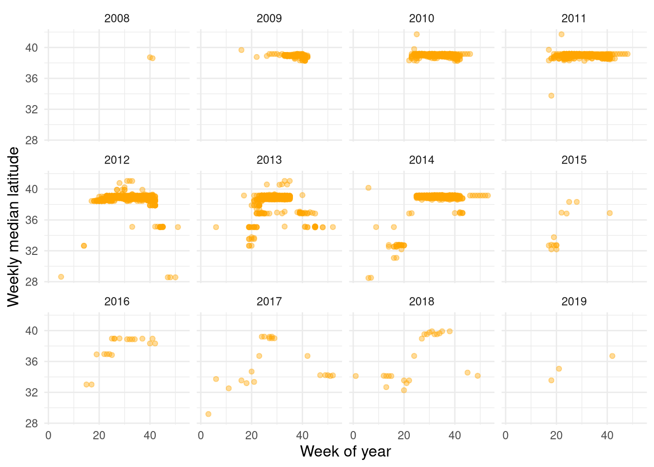
# A tibble: 1 × 2
   lon0  lat0
  <dbl> <dbl>
1 -75.1  38.7
proj_string <- paste0(
"+proj=aeqd +lon_0=",
round(projection_center$lon0, 3),
" +lat_0=",
round(projection_center$lat0, 3)
)
proj_string[1] "+proj=aeqd +lon_0=-75.117 +lat_0=38.743"sandtiger_sf <- sandtiger |>
st_as_sf(coords = c("med_lon", "med_lat"), crs = 4326) |>
st_transform(proj_string)
sandtiger_sf |>
distinct(geometry) |>
ggplot() +
geom_sf() +
coord_sf(datum = proj_string)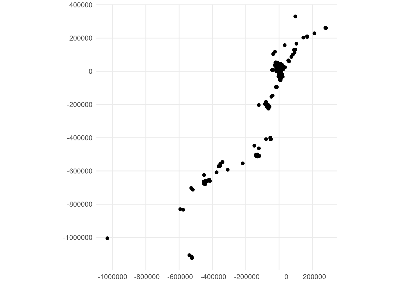
migration_azimuth <- sandtiger_sf |>
  # Extract AEQD coordinates
  st_coordinates() |>
  # Run PCA
  prcomp() |>
  # Extract PCA loadings
  _$rotation |>
  # Transpose matrix
  t() |>
  # Find coordinates of a second location on the X axis.
  # Here we use 1 km but it could be any value
  (\(.) c(1e3, 0) %*% .)() |>
  # Find the angle between true north and migration north
  (\(.) atan2(.[1], .[2]) * 180 / pi)()

# Measure clockwise from north
migration_azimuth <- ifelse(
  migration_azimuth < 0,
  180 + migration_azimuth,
  migration_azimuth
)

migration_azimuth
[1] 25.09121st_crs(sandtiger_sf) <- "+proj=aeqd +lat_0=90 +lon_0=0"
proj_rotated <- paste0("+proj=aeqd +lat_0=90 +lon_0=", migration_azimuth)
sandtiger_migration_north <- sandtiger_sf |>
st_transform(proj_rotated) |>
# extract coordinates for modeling purposes
mutate(x = st_coordinates(geometry)[, 1], y = st_coordinates(geometry)[, 2])
ggplot(sandtiger_migration_north) +
geom_sf() +
coord_sf(datum = proj_rotated)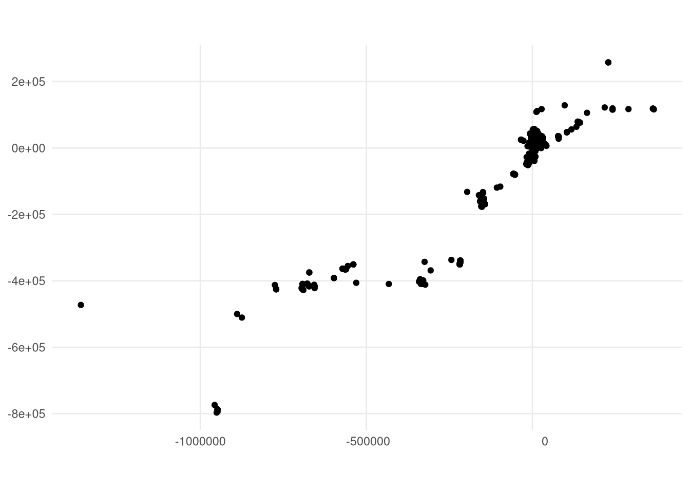
ggplot(sandtiger_migration_north) +
  geom_point(aes(x = wk, y = x), alpha = 0.4, color = "orange") +
  facet_wrap(~yr) +
  labs(
    title = "Migration synchrony",
    x = "Week of year",
    y = "Distance along the migration vector"
  ) +
  theme(axis.title = element_text(size = 12))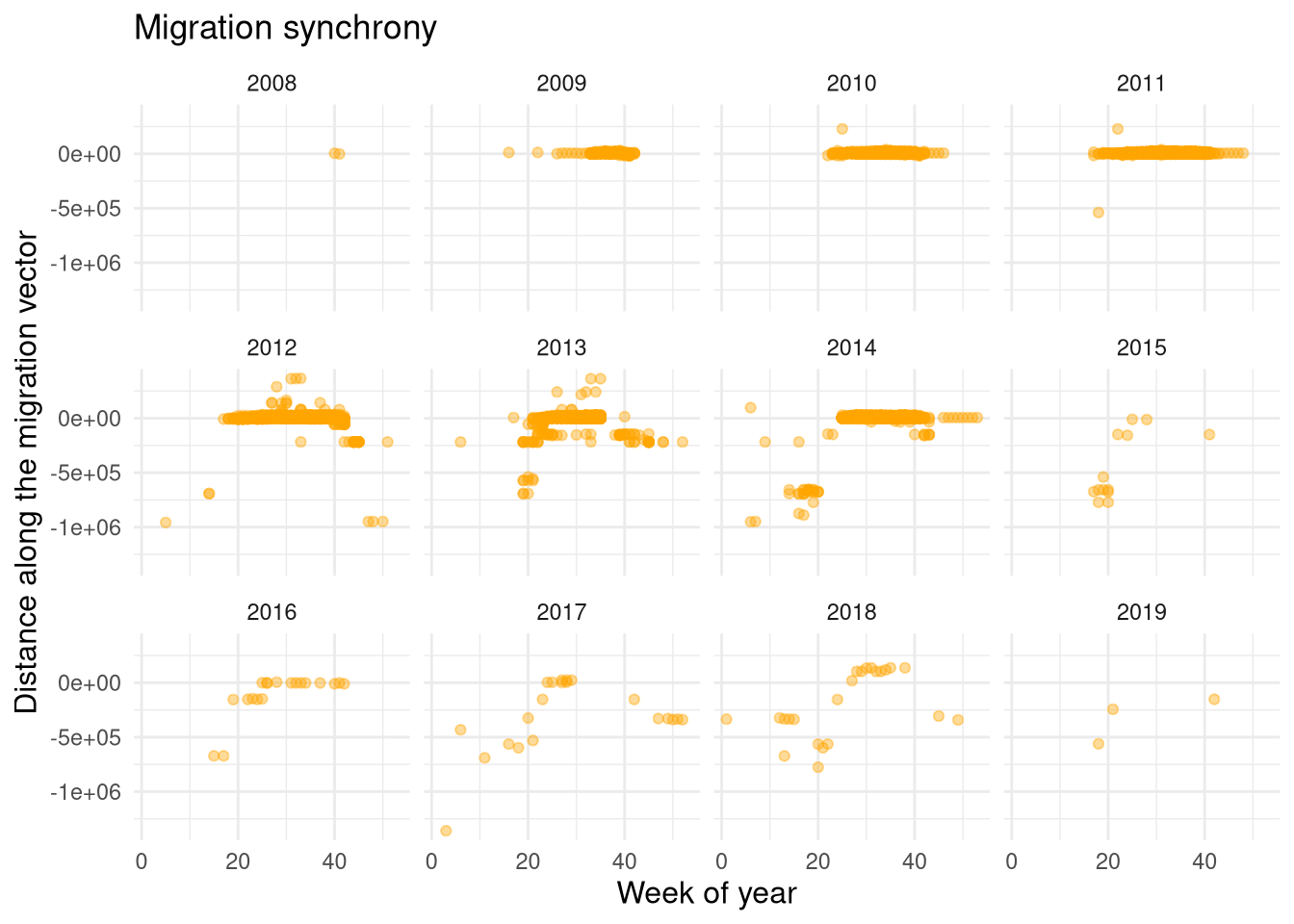
ggplot(sandtiger_migration_north) +
  geom_point(aes(x = wk, y = y, color = group), alpha = 0.4, color = "orange") +
  facet_wrap(~yr) +
  labs(
    title = "Migration front",
    x = "Week of year",
    y = "Distance across the migration vector"
  ) +
  theme(axis.title = element_text(size = 12))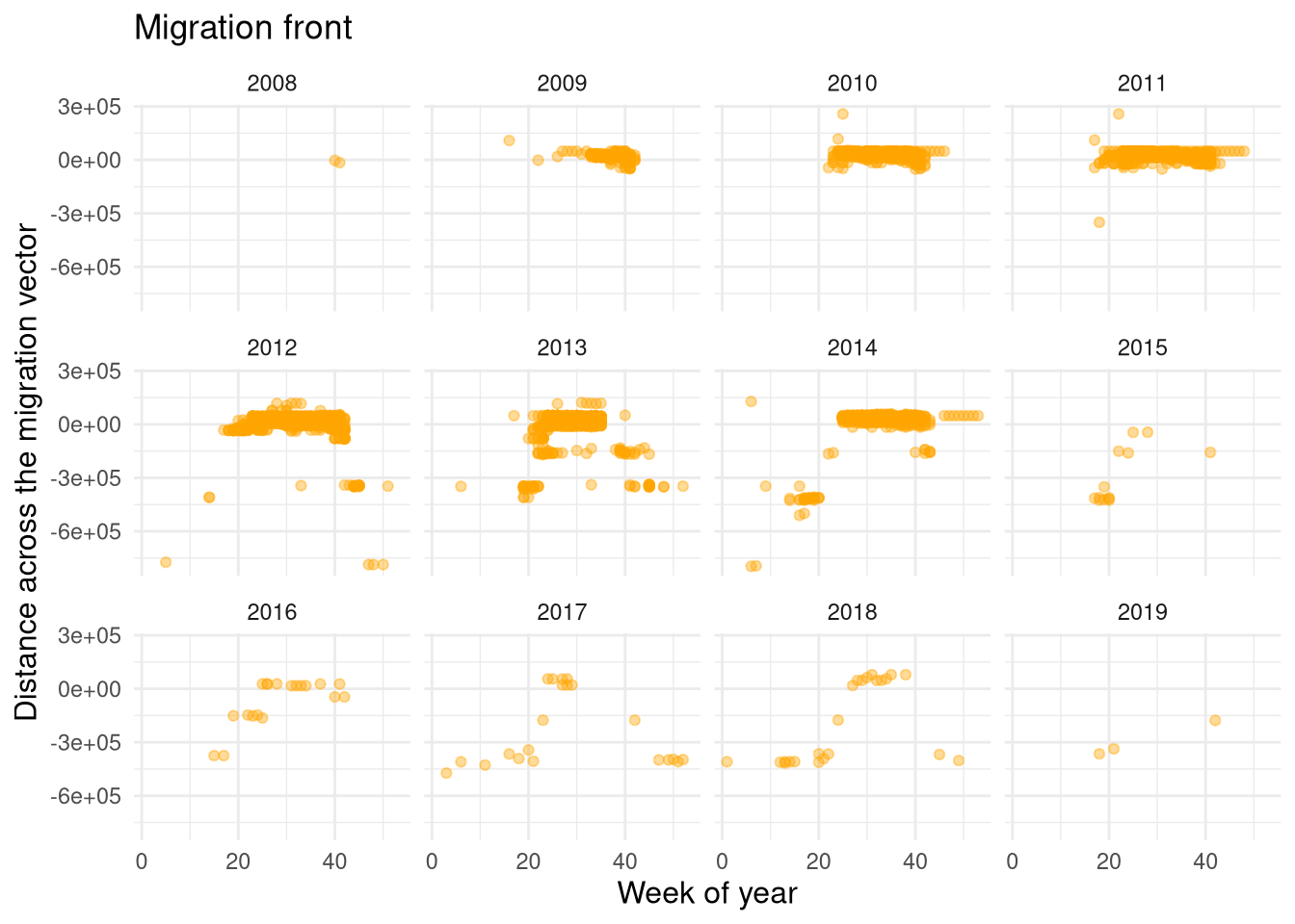
6.1.1 Initial GAM
6.1.1.1 Migration vector
model_data <- sandtiger_migration_north |>
  mutate(yr_f = factor(yr))

m1_st <- model_data |>
  gam(
    x ~ s(wk, k = 27, bs = "cc") + s(yr_f, bs = "re"),
    knots = list(wk = c(1, 53)),
    data = _,
    method = "REML"
  )

summary(m1_st)
Family: gaussian
Link function: identity

Formula:
x ~ s(wk, k = 27, bs = "cc") + s(yr_f, bs = "re")

Parametric coefficients:
            Estimate Std. Error t value Pr(>|t|)
(Intercept)   -55224      24767   -2.23   0.0258 *
---
Signif. codes:  0 '***' 0.001 '**' 0.01 '*' 0.05 '.' 0.1 ' ' 1

Approximate significance of smooth terms:
          edf Ref.df       F p-value
s(wk)   24.01     25 4328.72  <2e-16 ***
s(yr_f) 10.64     11   43.91  <2e-16 ***
---
Signif. codes:  0 '***' 0.001 '**' 0.01 '*' 0.05 '.' 0.1 ' ' 1

R-sq.(adj) =  0.574   Deviance explained = 57.7%
-REML = 71046 Scale est. = 2.9382e+09 n = 5759draw(m1_st, select = "s(wk)", residuals = TRUE)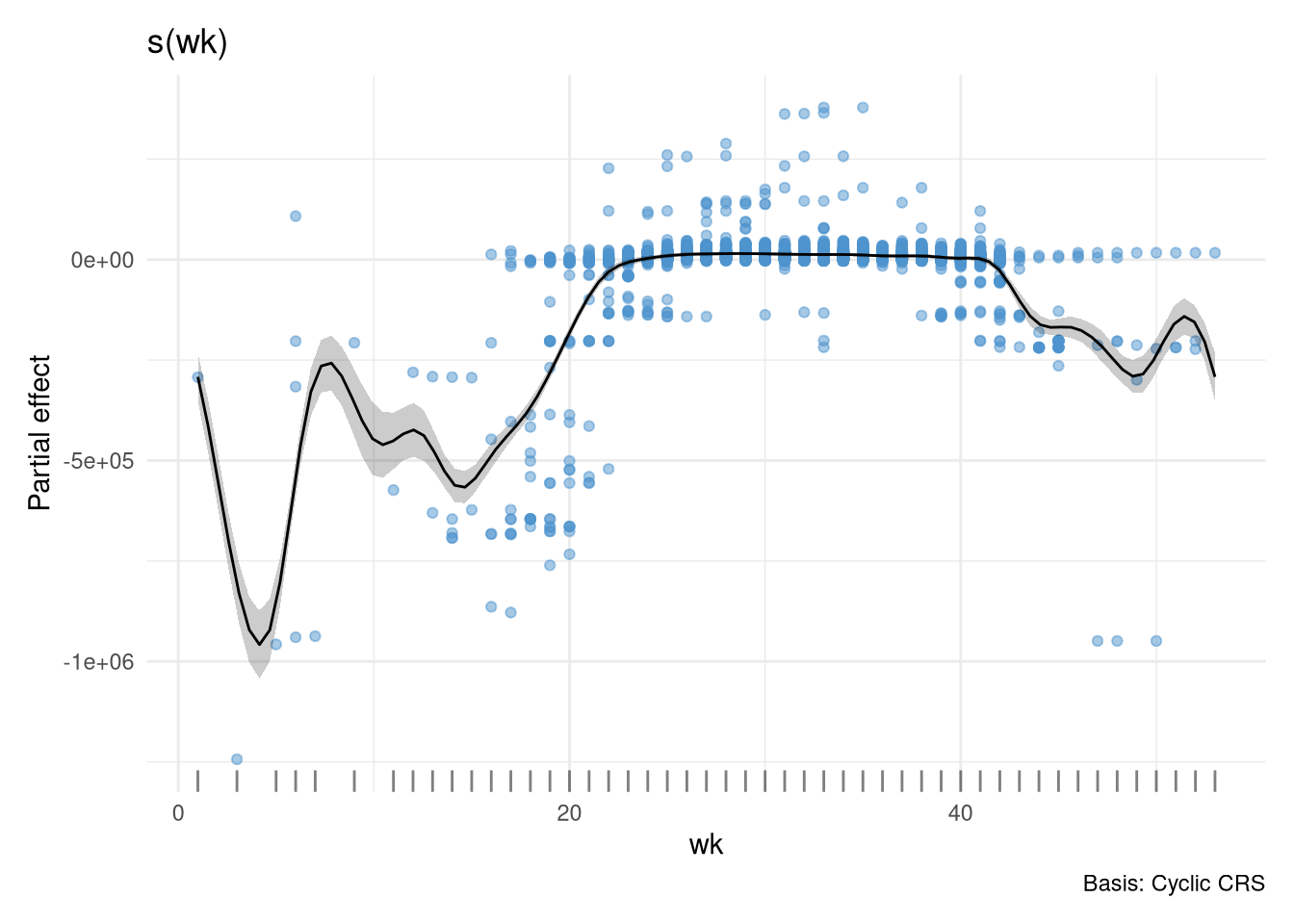
m2_st <- model_data |>
  gam(
    x ~ yr_f + s(wk, by = yr_f, k = 27, bs = "cc"),
    knots = list(wk = c(1, 53)),
    data = _,
    method = "REML"
  )


summary(m2_st)
Family: gaussian
Link function: identity

Formula:
x ~ yr_f + s(wk, by = yr_f, k = 27, bs = "cc")

Parametric coefficients:
             Estimate Std. Error t value Pr(>|t|)
(Intercept)    5237.4     1973.4   2.654  0.00798 **
yr_f2011       -321.4     2166.4  -0.148  0.88208
yr_f2013     -42477.6     3112.9 -13.645  < 2e-16 ***
yr_f2014     -20452.7     2331.6  -8.772  < 2e-16 ***
yr_f2012      -5507.1     2157.1  -2.553  0.01071 *
yr_f2010        277.5     2211.9   0.125  0.90017
yr_f2008      -3719.8    27071.3  -0.137  0.89071
yr_f2015    -122129.3   262896.7  -0.465  0.64227
yr_f2018      41996.4    15893.0   2.642  0.00825 **
yr_f2017      51717.8   452208.6   0.114  0.90895
yr_f2019      74448.6   219252.5   0.340  0.73420
yr_f2016     -25218.7    11448.8  -2.203  0.02765 *
---
Signif. codes:  0 '***' 0.001 '**' 0.01 '*' 0.05 '.' 0.1 ' ' 1

Approximate significance of smooth terms:
                     edf Ref.df       F  p-value
s(wk):yr_f2009  0.035947     14   0.000 0.934471
s(wk):yr_f2011  6.510823     20   1.297 0.000109 ***
s(wk):yr_f2013 18.143015     21 215.473  < 2e-16 ***
s(wk):yr_f2014 24.356384     25 599.666  < 2e-16 ***
s(wk):yr_f2012 20.902270     23 268.428  < 2e-16 ***
s(wk):yr_f2010  0.101991     16   0.005 0.432037
s(wk):yr_f2008  0.004463      3   0.000 0.888653
s(wk):yr_f2015  6.471024      8 147.123  < 2e-16 ***
s(wk):yr_f2018 13.014395     19 118.190  < 2e-16 ***
s(wk):yr_f2017 15.675741     18 141.659  < 2e-16 ***
s(wk):yr_f2019  1.962773      2  51.893  < 2e-16 ***
s(wk):yr_f2016 11.258557     16  54.144  < 2e-16 ***
---
Signif. codes:  0 '***' 0.001 '**' 0.01 '*' 0.05 '.' 0.1 ' ' 1

R-sq.(adj) =  0.874   Deviance explained = 87.7%
-REML = 67705 Scale est. = 8.7017e+08 n = 5759draw(m2_st, select = c("s(wk)"), partial_match = TRUE, residuals = TRUE)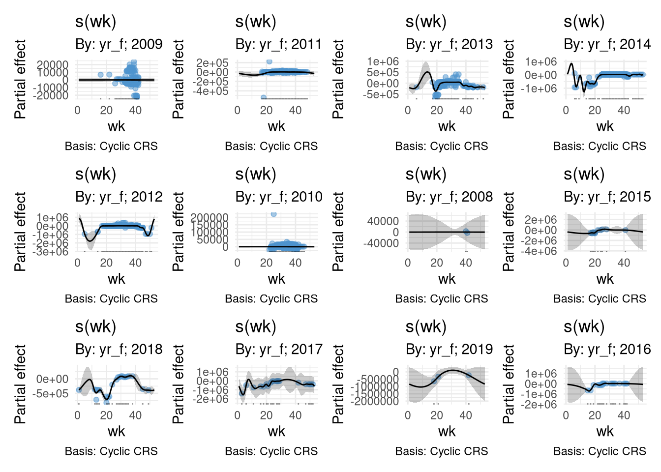
6.1.1.2 Migration front
We’ll do the same with the migration front (the deviation from the migration vector).
m1_mf <- model_data |>
  gam(
    y ~ s(wk, k = 27, bs = "cc") + s(yr_f, bs = "re"),
    knots = list(wk = c(1, 53)),
    data = _,
    method = "REML"
  )

summary(m1_mf)
Family: gaussian
Link function: identity

Formula:
y ~ s(wk, k = 27, bs = "cc") + s(yr_f, bs = "re")

Parametric coefficients:
            Estimate Std. Error t value Pr(>|t|)
(Intercept)   -29480      18807  -1.568    0.117

Approximate significance of smooth terms:
          edf Ref.df       F p-value
s(wk)   21.36     25 4167.30  <2e-16 ***
s(yr_f) 10.58     11   45.34  <2e-16 ***
---
Signif. codes:  0 '***' 0.001 '**' 0.01 '*' 0.05 '.' 0.1 ' ' 1

R-sq.(adj) =  0.598   Deviance explained =   60%
-REML = 69922 Scale est. = 2.0046e+09 n = 5759draw(m1_mf, select = "s(wk)", residuals = TRUE)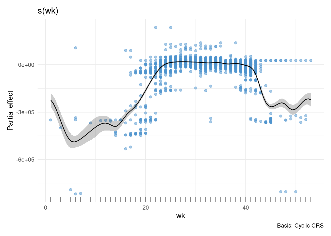
m2_mf <- model_data |>
  gam(
    y ~ yr_f + yr_f + s(wk, by = yr_f, k = 27, bs = "cc"),
    knots = list(wk = c(1, 53)),
    data = _,
    method = "REML"
  )

summary(m2_mf)
Family: gaussian
Link function: identity

Formula:
y ~ yr_f + yr_f + s(wk, by = yr_f, k = 27, bs = "cc")

Parametric coefficients:
             Estimate Std. Error t value Pr(>|t|)
(Intercept)   29397.8     3671.6   8.007 1.42e-15 ***
yr_f2011      -3948.4     3761.5  -1.050 0.293909
yr_f2013     -56068.8     4319.1 -12.982  < 2e-16 ***
yr_f2014     -12463.7     3841.2  -3.245 0.001182 **
yr_f2012     -13519.1     3745.4  -3.610 0.000309 ***
yr_f2010       -198.6     3964.9  -0.050 0.960059
yr_f2008     -38222.2    33346.1  -1.146 0.251750
yr_f2015    -124464.3    82008.5  -1.518 0.129146
yr_f2018     -28914.0    10141.0  -2.851 0.004371 **
yr_f2017     -59549.6    74722.2  -0.797 0.425516
yr_f2019    -271979.3    45919.4  -5.923 3.35e-09 ***
yr_f2016     -32481.3     9276.1  -3.502 0.000466 ***
---
Signif. codes:  0 '***' 0.001 '**' 0.01 '*' 0.05 '.' 0.1 ' ' 1

Approximate significance of smooth terms:
                    edf Ref.df       F  p-value
s(wk):yr_f2009  2.70670     14   1.612 7.75e-06 ***
s(wk):yr_f2011  7.35684     20   5.225  < 2e-16 ***
s(wk):yr_f2013 18.67490     21 369.195  < 2e-16 ***
s(wk):yr_f2014 23.80834     25 356.027  < 2e-16 ***
s(wk):yr_f2012 20.52964     23 322.082  < 2e-16 ***
s(wk):yr_f2010  8.36187     16   4.589  < 2e-16 ***
s(wk):yr_f2008  0.01339      4   0.000    0.742
s(wk):yr_f2015  5.10558      8  47.384  < 2e-16 ***
s(wk):yr_f2018  9.47040     19  81.634  < 2e-16 ***
s(wk):yr_f2017 11.28888     18  66.331  < 2e-16 ***
s(wk):yr_f2019  1.37134      3   8.950 1.99e-07 ***
s(wk):yr_f2016  7.84278     16  23.450  < 2e-16 ***
---
Signif. codes:  0 '***' 0.001 '**' 0.01 '*' 0.05 '.' 0.1 ' ' 1

R-sq.(adj) =  0.855   Deviance explained = 85.8%
-REML = 67116 Scale est. = 7.2302e+08 n = 5759draw(m2_mf, select = "s(wk)", residuals = TRUE, partial_match = TRUE)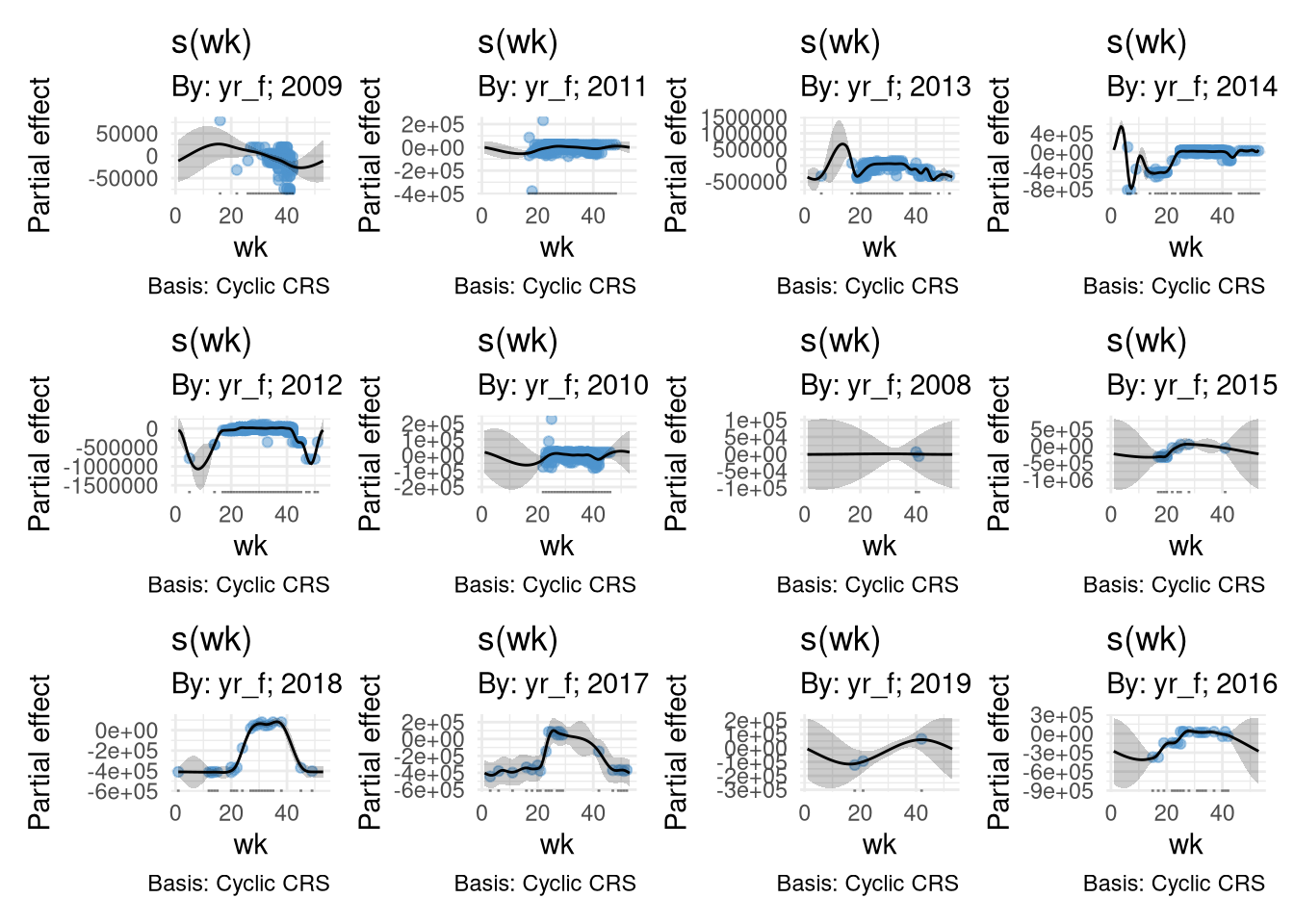
6.1.2 Model evaluation
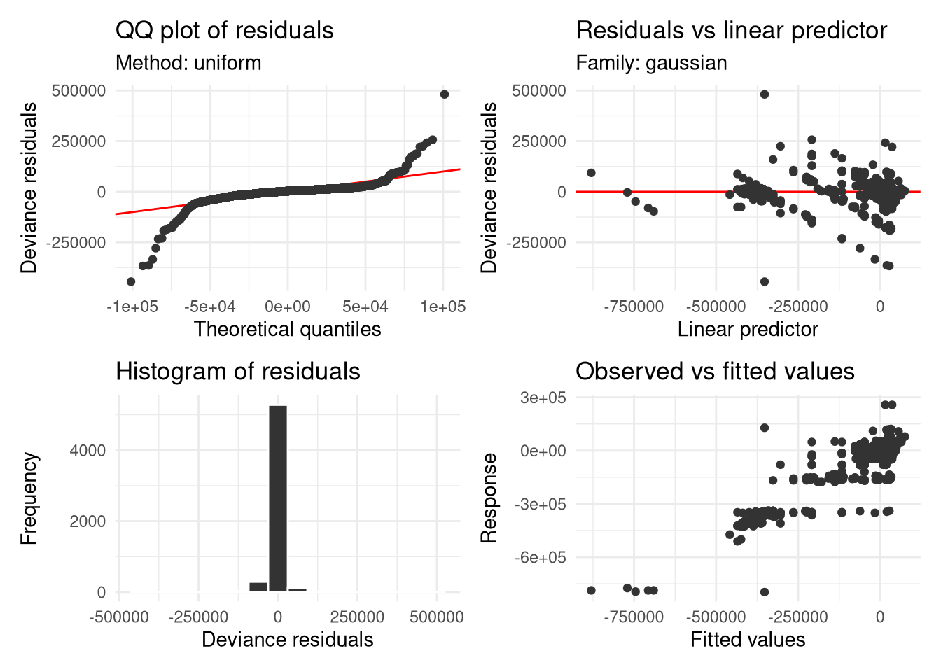
appraise(m1_st)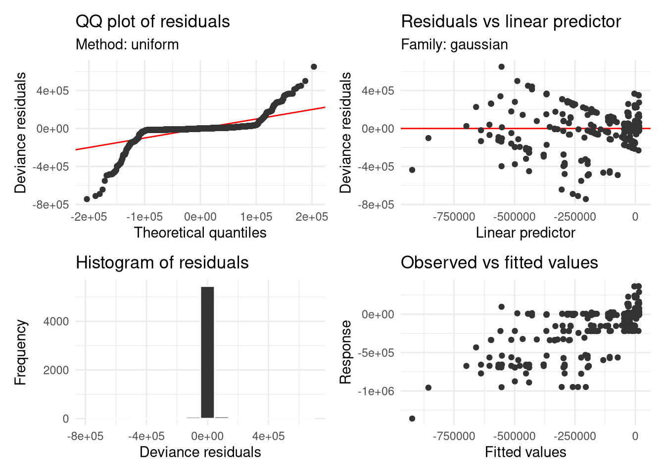
appraise(m2_st)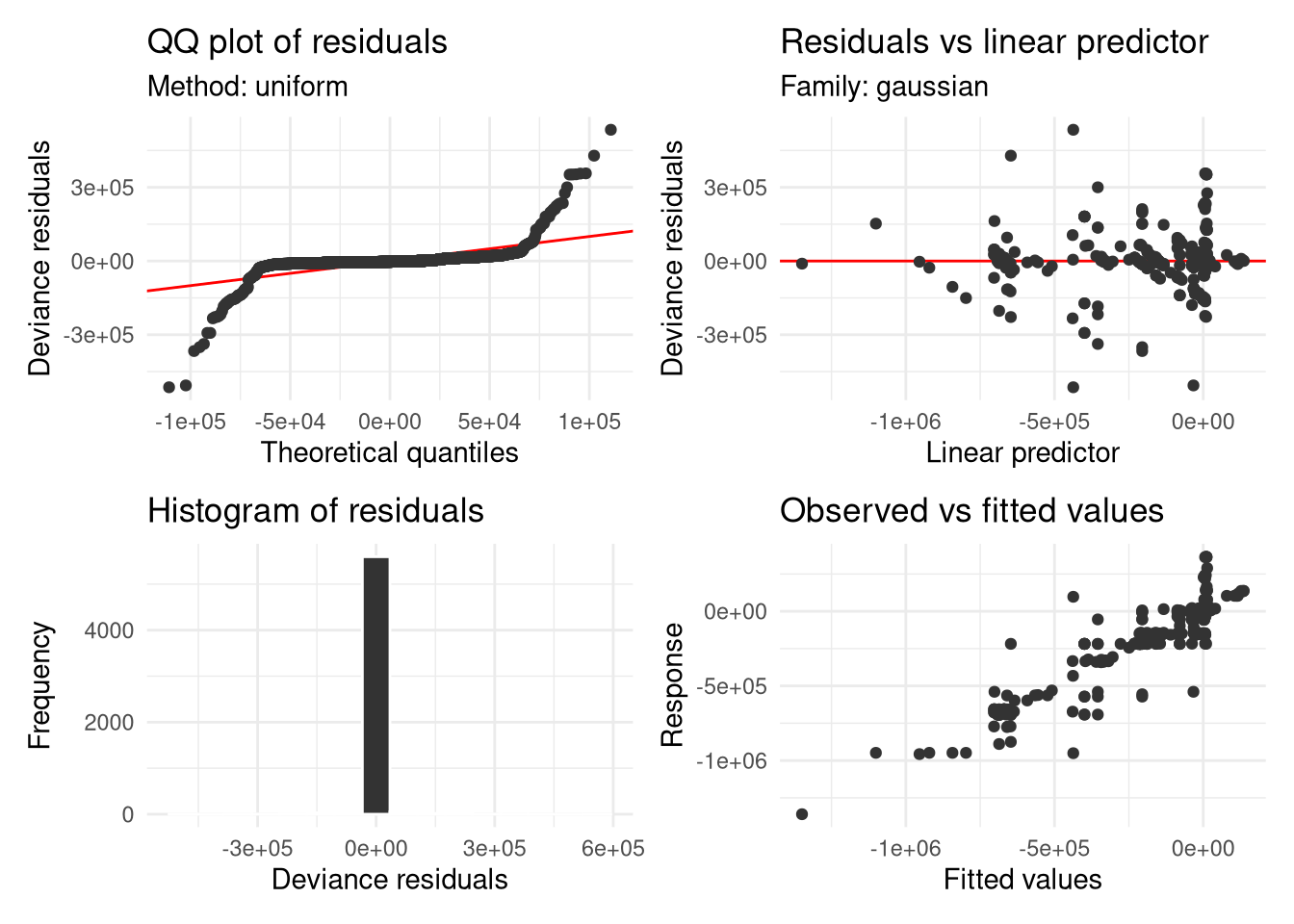
appraise(m1_mf)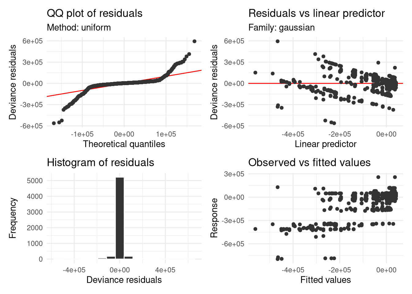
appraise(m2_mf)