library(arrow) # Data import
library(dplyr) # Data manipulation
library(sf) # Spatial
library(ggplot2) # Data visualization
library(mgcv) # GAM fitting
library(gratia) # GAM visualization

theme_set(theme_minimal())5 Initial striped bass GAM exploration
Let’s take a look at striped bass Morone saxatilis using the data prepared in the data cleaning chapter.
We first visualize the distribution of the median per-individual latitudes through time:
ggplot(sb) +
  geom_point(aes(x = wk, y = med_lat, color = group), alpha = 0.4) +
  facet_wrap(~year) +
  labs(x = "Week of year", y = "Weekly median latitude") +
  theme(axis.title = element_text(size = 12))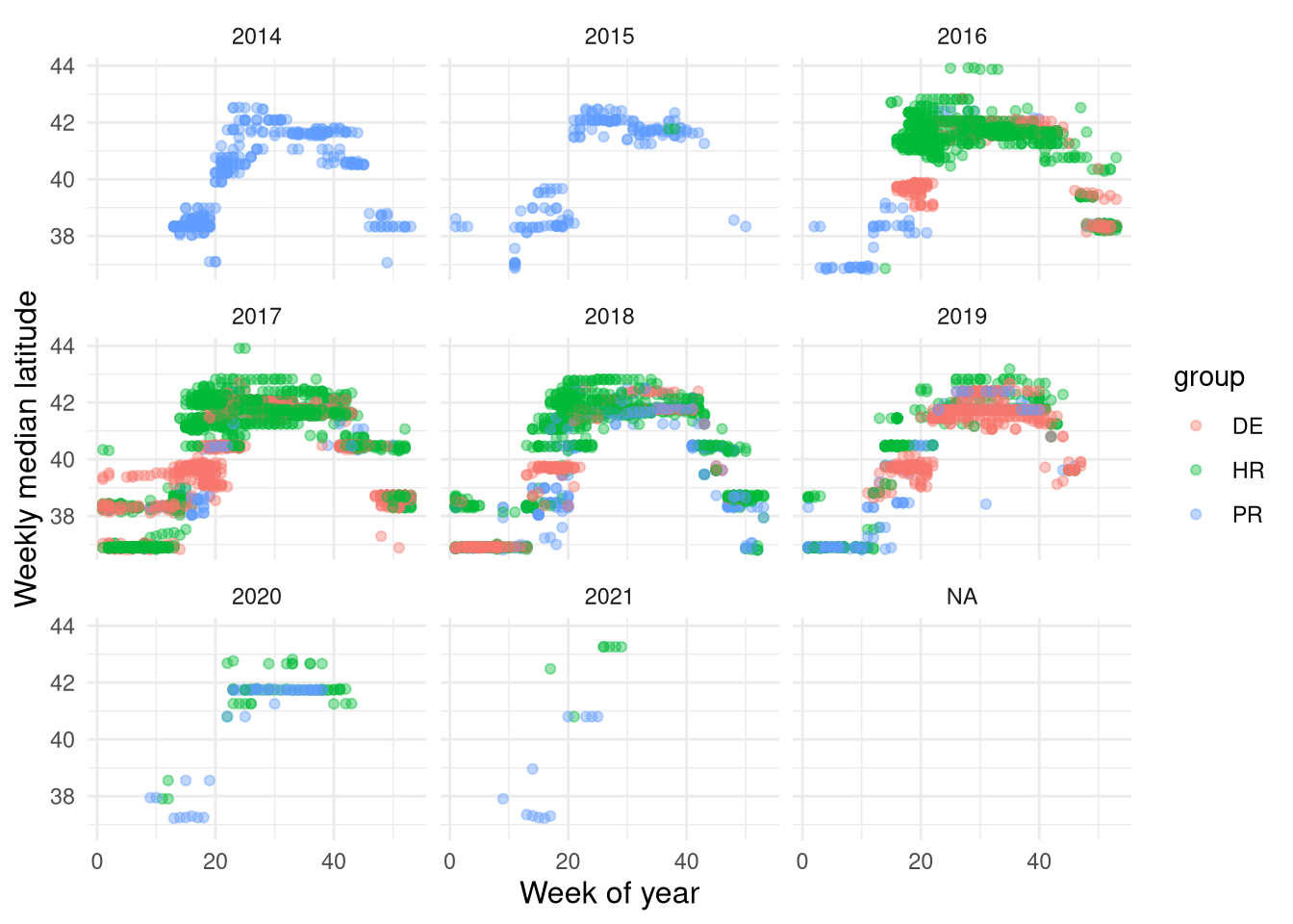
Following our projectiong selection procedure in the Projection Error chapter, we project the data into an azimuthal equidistant projection (AEQD) and rotate the data to “migration north”. To project into AEQD, we first need a projection center. This will be the median receiver location.
# A tibble: 1 × 2
   lon0  lat0
  <dbl> <dbl>
1 -73.9  40.6
Create the PROJ string…
proj_string <- paste0(
  "+proj=aeqd +lon_0=",
  round(projection_center$lon0, 3),
  " +lat_0=",
  round(projection_center$lat0, 3)
)

proj_string
[1] "+proj=aeqd +lon_0=-73.9 +lat_0=40.601"…and project the fish locations:
sb_sf <- sb |>
  st_as_sf(coords = c("med_lon", "med_lat"), crs = 4326, remove = FALSE) |>
  st_transform(proj_string)

sb_sf |>
  distinct(med_lon, med_lat, .keep_all = TRUE) |>
  ggplot() +
  geom_sf() +
  coord_sf(datum = proj_string)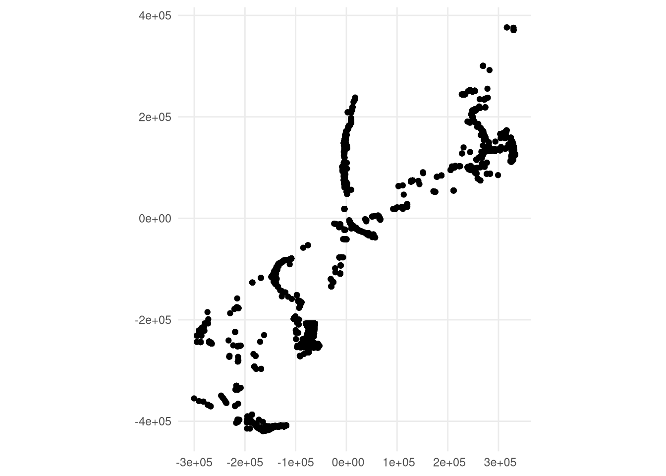
We now conduct principle components analysis (PCA) on the major migration vector to find its angle from true north: the migration azimuth.
migration_azimuth <- sb_sf |>
  # Extract AEQD coordinates
  st_coordinates() |>
  # Run PCA
  prcomp() |>
  # Extract PCA loadings
  _$rotation |>
  # Transpose matrix
  t() |>
  # Find coordinates of a second location on the X axis.
  # Here we use 1 km but it could be any value
  (\(.) c(1e3, 0) %*% .)() |>
  # Find the angle between true north and migration north
  (\(.) atan2(.[1], .[2]) * 180 / pi)()

# Measure clockwise from north
migration_azimuth <- ifelse(
  migration_azimuth < 0,
  180 + migration_azimuth,
  migration_azimuth
)
So, the migration vector is rotated 43\(\degree\) from north. To rotate the data, we’re going to lie to the program and say that the data are currently projected around the north pole, then add the migration azimuth to it.
st_crs(sb_sf) <- "+proj=aeqd +lat_0=90 +lon_0=0"
proj_rotated <- paste0("+proj=aeqd +lat_0=90 +lon_0=", migration_azimuth)

sb_migration_north <- sb_sf |>
  st_transform(proj_rotated) |>
  # extract coordinates for modeling purposes
  mutate(x = st_coordinates(geometry)[, 1], y = st_coordinates(geometry)[, 2])


ggplot(sb_migration_north) +
  geom_sf() +
  coord_sf(datum = proj_rotated)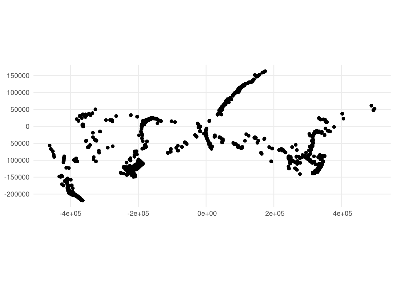
We can now visualize migration synchrony, the variance in the migration vector over time, and migration front, variance in excursion from the migration vector over time (Secor et al. 2025).
ggplot(sb_migration_north) +
  geom_point(aes(x = wk, y = x, color = group), alpha = 0.4) +
  facet_wrap(~year) +
  labs(
    title = "Migration synchrony",
    x = "Week of year",
    y = "Distance along the migration vector"
  ) +
  theme(axis.title = element_text(size = 12))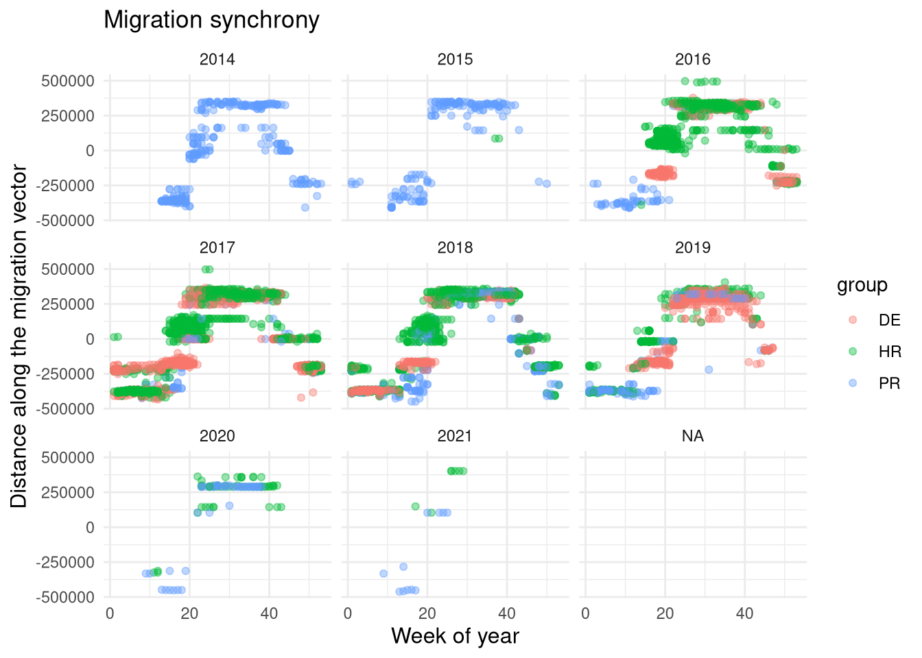
ggplot(sb_migration_north) +
  geom_point(aes(x = wk, y = y, color = group), alpha = 0.4) +
  facet_wrap(~year) +
  labs(
    title = "Migration front",
    x = "Week of year",
    y = "Distance across the migration vector"
  ) +
  theme(axis.title = element_text(size = 12))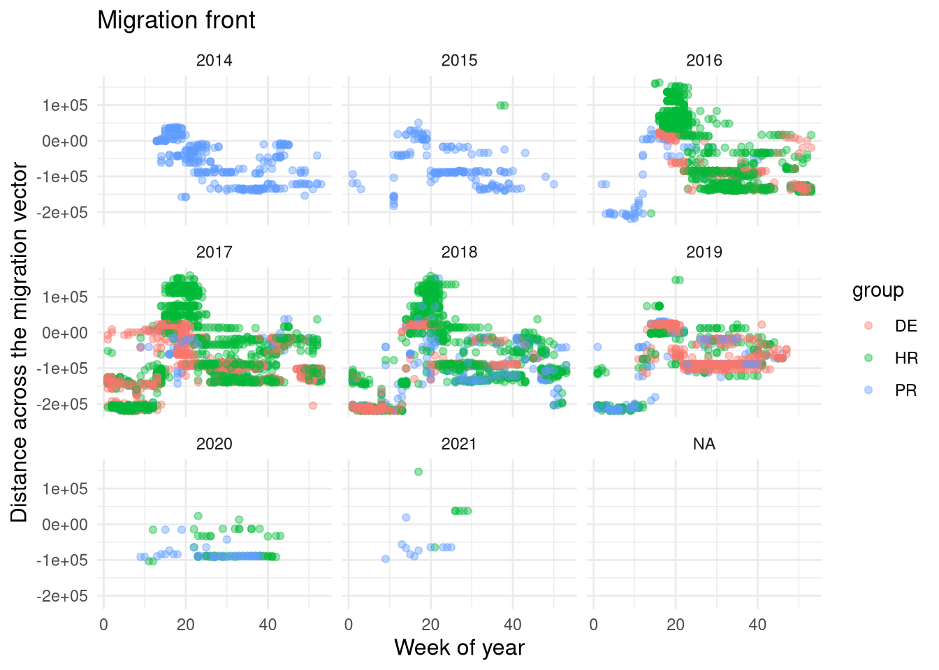
5.0.1 Initial GAM
5.0.1.1 Migration vector
For the initial GAM, we’ll treat both year and population as a random effect. We see a general trend of low values on the migration vector through the beginning of the year, a rapid increase after the 10th week, a slight reduction in rate in week 15-20, then another rapid increase through week 25. Posiiton then levels off through week 40, where it rapidly drops.
model_data <- sb_migration_north |>
  mutate(group = factor(group), yr_f = factor(year))

m1 <- model_data |>
  gam(
    x ~ s(wk, k = 27, bs = "cc") + s(yr_f, bs = "re") + s(group, bs = "re"),
    knots = list(wk = c(1, 53)),
    data = _,
    method = "REML"
  )

summary(m1)
Family: gaussian
Link function: identity

Formula:
x ~ s(wk, k = 27, bs = "cc") + s(yr_f, bs = "re") + s(group,
    bs = "re")

Parametric coefficients:
            Estimate Std. Error t value Pr(>|t|)
(Intercept)    17025      25040    0.68    0.497

Approximate significance of smooth terms:
            edf Ref.df       F p-value
s(wk)    20.768     25 15255.0  <2e-16 ***
s(yr_f)   6.178      7   158.5  <2e-16 ***
s(group)  1.993      2  1481.8  <2e-16 ***
---
Signif. codes:  0 '***' 0.001 '**' 0.01 '*' 0.05 '.' 0.1 ' ' 1

R-sq.(adj) =  0.877   Deviance explained = 87.7%
-REML = 95557 Scale est. = 8.5289e+09 n = 7431draw(m1, select = "s(wk)", residuals = TRUE)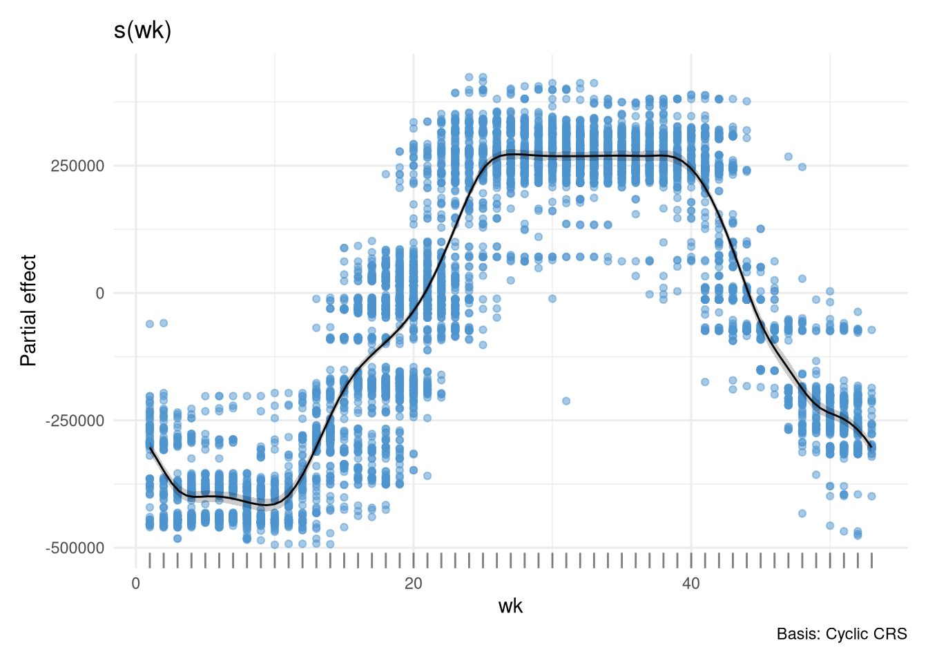
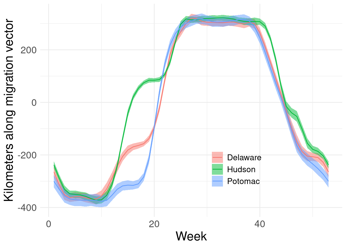
Next we’ll pull the populations apart and treat them as “by-variable smooths” (i.e. one form of a GAM interaction) in the model. We see that the leveling-off of movement up the migration vector in weeks 15-20 is likely due to spawning. The Potomac River has a leveling-off earlier and lower on the vector, followed by Delaware a little higher and later, then Hudson higher and greater still. These destination habitats are one of the migration metrics we wish to quantify.
m2 <- model_data |>
  # rename "group" variable; we'll use the marginaleffects library soon and
  #   "group" makes the program confused
  mutate(grp = group) |>
  gam(
    x ~ grp + s(wk, by = grp, k = 27, bs = "cc") + s(yr_f, bs = "re"),
    knots = list(wk = c(1, 53)),
    data = _,
    method = "REML"
  )


summary(m2)
Family: gaussian
Link function: identity

Formula:
x ~ grp + s(wk, by = grp, k = 27, bs = "cc") + s(yr_f, bs = "re")

Parametric coefficients:
            Estimate Std. Error t value Pr(>|t|)
(Intercept)    69079       6060   11.40   <2e-16 ***
grpPR         -84156       3061  -27.49   <2e-16 ***
grpDE         -60663       2190  -27.70   <2e-16 ***
---
Signif. codes:  0 '***' 0.001 '**' 0.01 '*' 0.05 '.' 0.1 ' ' 1

Approximate significance of smooth terms:
               edf Ref.df       F p-value
s(wk):grpHR 22.729     25 3029.34  <2e-16 ***
s(wk):grpPR 18.788     25  714.34  <2e-16 ***
s(wk):grpDE 19.868     25 1838.69  <2e-16 ***
s(yr_f)      5.955      7   10.55  <2e-16 ***
---
Signif. codes:  0 '***' 0.001 '**' 0.01 '*' 0.05 '.' 0.1 ' ' 1

R-sq.(adj) =  0.912   Deviance explained = 91.3%
-REML = 94348 Scale est. = 6.0601e+09 n = 7431draw(m2, select = c("s(wk)"), partial_match = TRUE, residuals = TRUE)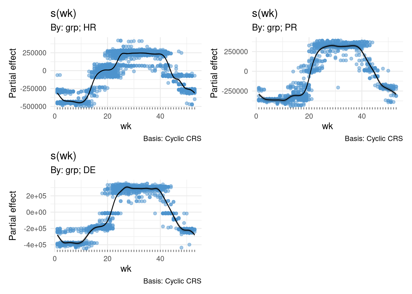
It’s a bit more interesting if these curves are overplotted. We’ll use the marginaleffects package to marginalize out random effects.
library(marginaleffects)
m2_preds <- predictions(
  m2,
  newdata = datagrid(wk = 1:53, grp = c("HR", "PR", "DE")),
  condition = c("wk", "grp"),
  exclude = "yr_f"
) |>
  mutate(
    system = case_when(
      grepl("HR", grp) ~ "Hudson",
      grepl("PR", grp) ~ "Potomac",
      grepl("DE", grp) ~ "Delaware"
    )
  )

ggplot(m2_preds) +
  geom_ribbon(
    aes(x = wk, ymin = conf.low / 1000, ymax = conf.high / 1000, fill = system),
    alpha = 0.5
  ) +
  geom_line(aes(x = wk, y = estimate / 1000, color = system)) +
  labs(
    x = "Week",
    y = "Kilometers along migration vector",
    fill = "",
    color = ""
  ) +
  theme(
    axis.text = element_text(size = 14),
    axis.title = element_text(size = 18),
    legend.text = element_text(size = 12),
    legend.position = "inside",
    legend.position.inside = c(0.65, 0.25)
  )
5.0.1.1.1 Derivatives
m2_d <- derivatives(m2, select = "s(wk)", partial_match = T, n = 52) |>
  mutate(
    system = case_when(
      grepl("HR", .smooth) ~ "Hudson",
      grepl("PR", .smooth) ~ "Potomac",
      grepl("DE", .smooth) ~ "Delaware"
    )
  )

draw(m2_d)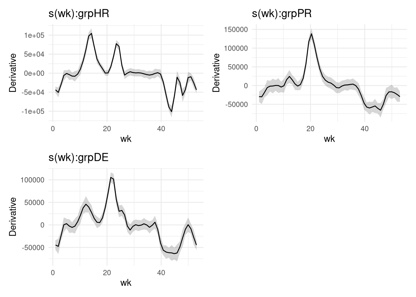
m2_d |>
  ggplot() +
  geom_ribbon(
    aes(
      x = wk,
      ymin = .lower_ci / 1000,
      ymax = .upper_ci / 1000,
      fill = system
    ),
    alpha = 0.5
  ) +
  geom_line(aes(x = wk, y = .derivative / 1000, color = system)) +
  labs(
    x = "Week",
    y = "Migration velocity (km/week)",
    fill = "System",
    color = "System"
  ) +
  theme(
    axis.text = element_text(size = 14),
    axis.title = element_text(size = 18),
    legend.text = element_text(size = 12),
    legend.title = element_text(size = 12),
    legend.position = "inside",
    legend.position.inside = c(0.7, 0.7)
  )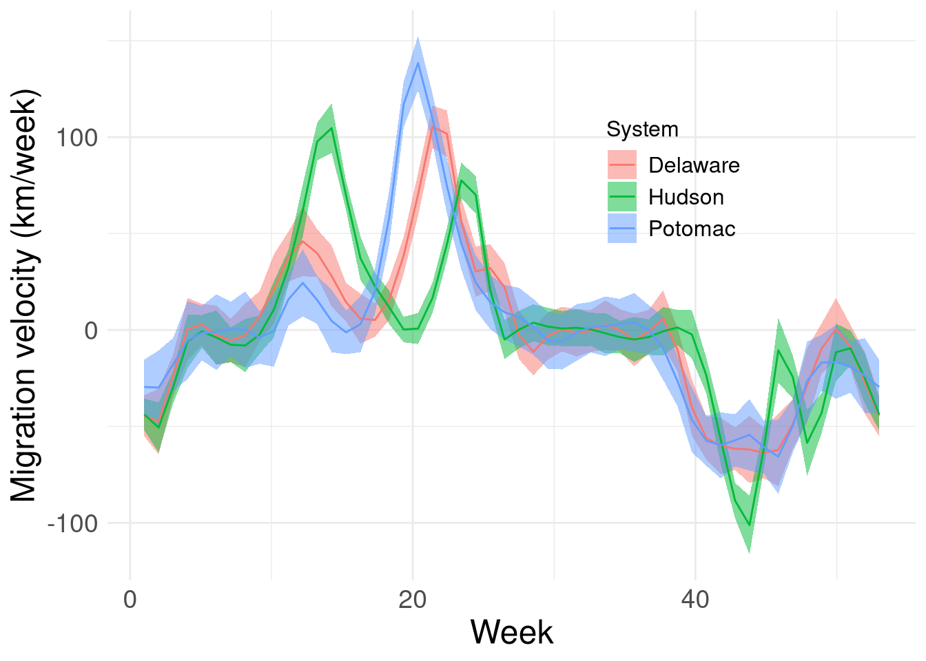
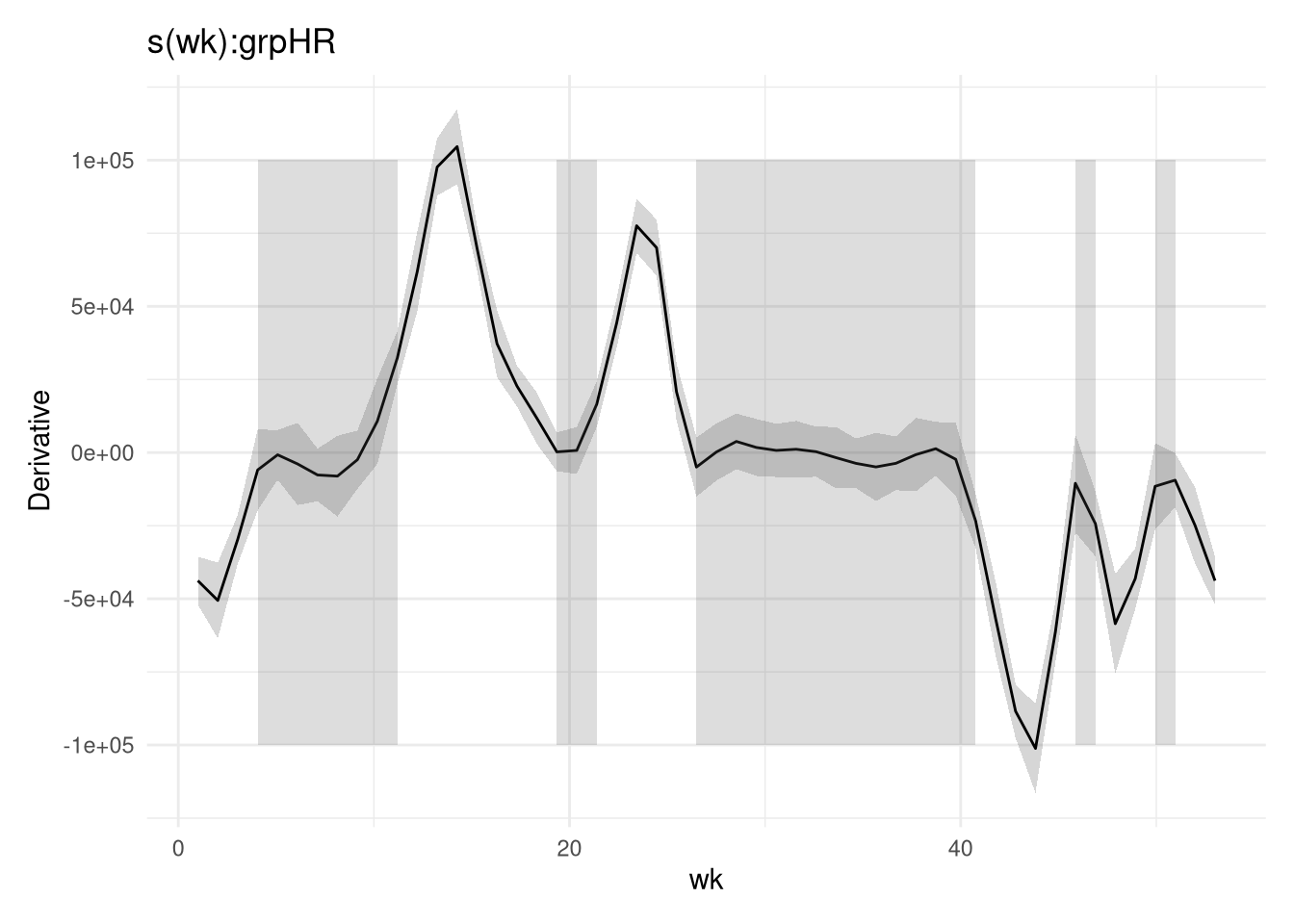
What might a migration metric look like? If we define a “destination habitat” as a time when \(d/d(wk) \approx 0\), here are the locations where Hudson River fish might at their destination habitat:
hr_dest_hab <- m2_d |>
  group_by(grp) |>
  mutate(
    zero = (.lower_ci <= 0 & .upper_ci >= 0),
    id = consecutive_id(zero)
  ) |>
  filter(id != 1, grp == "HR") |>
  distinct(zero, id, .keep_all = TRUE) |>
  mutate(id = rep(1:(n() / 2), each = 2)) |>
  tidyr::pivot_wider(id_cols = id, names_from = zero, values_from = wk)

draw(m2_d, select = "s(wk):grpHR") +
  annotate(
    "rect",
    xmin = hr_dest_hab$`TRUE`,
    xmax = hr_dest_hab$`FALSE`,
    ymin = -1e5,
    ymax = 1e5,
    alpha = 0.2
  )
5.0.1.2 Migration front
We’ll do the same with the migration front (the deviation from the migration vector).
m1_mf <- model_data |>
  gam(
    y ~ s(wk, k = 53, bs = "cc") +
      s(yr_f, bs = "re") +
      s(group, bs = "re"),
    knots = list(wk = c(1, 53)),
    data = _,
    method = "REML"
  )

summary(m1_mf)
Family: gaussian
Link function: identity

Formula:
y ~ s(wk, k = 53, bs = "cc") + s(yr_f, bs = "re") + s(group,
    bs = "re")

Parametric coefficients:
            Estimate Std. Error t value Pr(>|t|)
(Intercept)   -72156       6320  -11.42   <2e-16 ***
---
Signif. codes:  0 '***' 0.001 '**' 0.01 '*' 0.05 '.' 0.1 ' ' 1

Approximate significance of smooth terms:
            edf Ref.df       F p-value
s(wk)    33.092     51 453.854 < 2e-16 ***
s(yr_f)   4.197      7   8.521 0.00755 **
s(group)  1.975      2 172.261 < 2e-16 ***
---
Signif. codes:  0 '***' 0.001 '**' 0.01 '*' 0.05 '.' 0.1 ' ' 1

R-sq.(adj) =  0.722   Deviance explained = 72.3%
-REML = 90614 Scale est. = 2.2479e+09 n = 7431draw(m1_mf, select = "s(wk)", residuals = TRUE)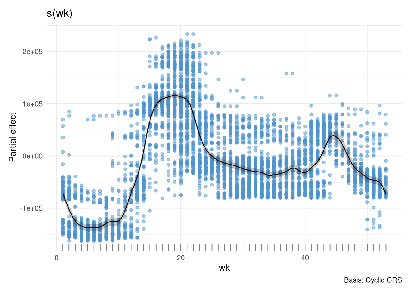
m2_mf <- model_data |>
  mutate(grp = group) |>
  gam(
    y ~ grp +
      s(wk, by = grp, k = 53, bs = "cc") +
      s(yr_f, bs = "re"),
    knots = list(wk = c(1, 53)),
    data = _,
    method = "REML"
  )

summary(m2_mf)
Family: gaussian
Link function: identity

Formula:
y ~ grp + s(wk, by = grp, k = 53, bs = "cc") + s(yr_f, bs = "re")

Parametric coefficients:
            Estimate Std. Error t value Pr(>|t|)
(Intercept)   -57394       2554  -22.47   <2e-16 ***
grpPR         -24870       1626  -15.29   <2e-16 ***
grpDE         -18398       1176  -15.64   <2e-16 ***
---
Signif. codes:  0 '***' 0.001 '**' 0.01 '*' 0.05 '.' 0.1 ' ' 1

Approximate significance of smooth terms:
               edf Ref.df      F p-value
s(wk):grpHR 34.048     51 535.43  <2e-16 ***
s(wk):grpPR 19.894     51  49.60  <2e-16 ***
s(wk):grpDE 22.237     51 100.04  <2e-16 ***
s(yr_f)      5.518      7  13.63  <2e-16 ***
---
Signif. codes:  0 '***' 0.001 '**' 0.01 '*' 0.05 '.' 0.1 ' ' 1

R-sq.(adj) =  0.783   Deviance explained = 78.6%
-REML = 89740 Scale est. = 1.75e+09 n = 7431draw(m2_mf, select = "s(wk)", partial_match = TRUE, residuals = TRUE)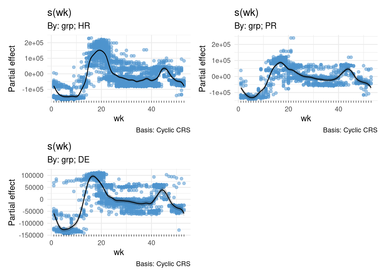
library(marginaleffects)
j <- predictions(
  m2_mf,
  newdata = datagrid(wk = 1:53, grp = c("HR", "PR", "DE")),
  condition = c("wk", "grp"),
  exclude = "yr_f"
)

j |>
  mutate(
    system = case_when(
      grepl("HR", grp) ~ "Hudson",
      grepl("PR", grp) ~ "Potomac",
      grepl("DE", grp) ~ "Delaware"
    )
  ) |>

  ggplot() +
  geom_ribbon(
    aes(x = wk, ymin = conf.low / 1000, ymax = conf.high / 1000),
    fill = "gray"
  ) +
  geom_line(aes(x = wk, y = estimate / 1000)) +
  labs(x = "Week", y = "Kilometers across migration vector") +
  facet_wrap(~system, ncol = 2)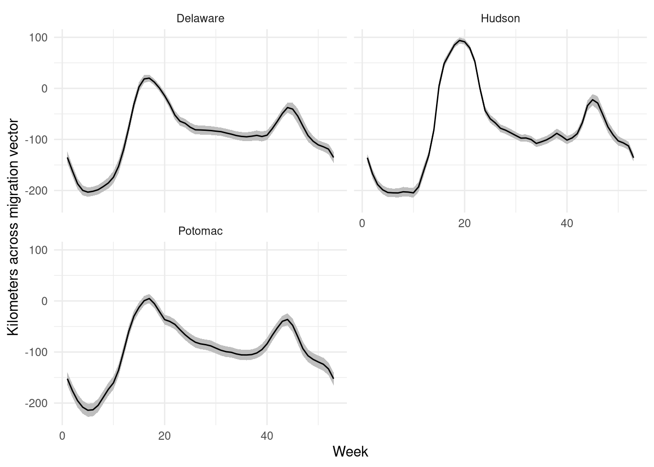
m2f_d <- derivatives(m2_mf, select = "s(wk)", partial_match = T, n = 53)

m2f_d |>
  mutate(
    system = case_when(
      grepl("HR", .smooth) ~ "Hudson",
      grepl("PR", .smooth) ~ "Potomac",
      grepl("DE", .smooth) ~ "Delaware"
    )
  ) |>
  ggplot() +
  geom_ribbon(
    aes(x = wk, ymin = .lower_ci / 1000, ymax = .upper_ci / 1000),
    fill = 'gray'
  ) +
  geom_line(aes(x = wk, y = .derivative / 1000)) +
  facet_wrap(~system, nrow = 2) +
  labs(x = "Week", y = "Migration front velocity (km/week)")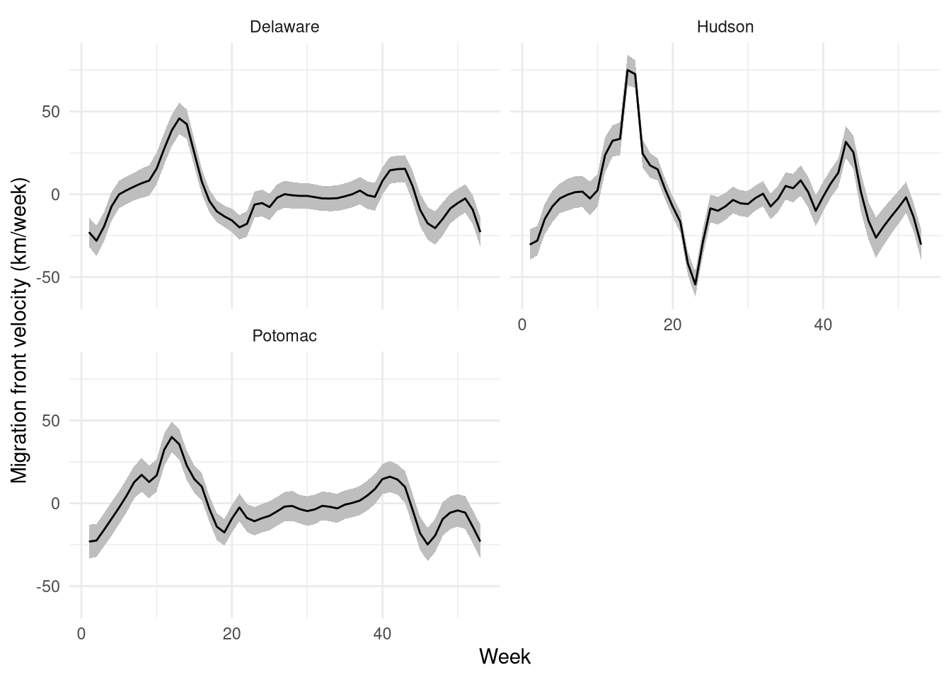
5.0.2 Model evaluation
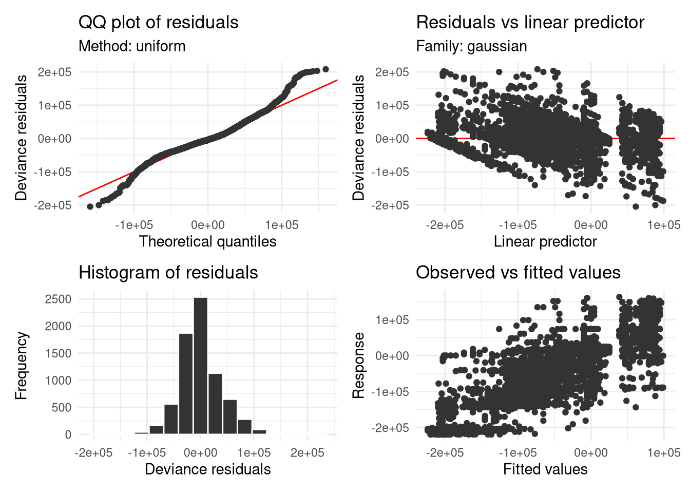
It should be noted, however, that the initial models are not performing well on the edges of the domain of the migration vector and migration front. This suggests that we need to refine the model to further to characterize these areas.
appraise(m1)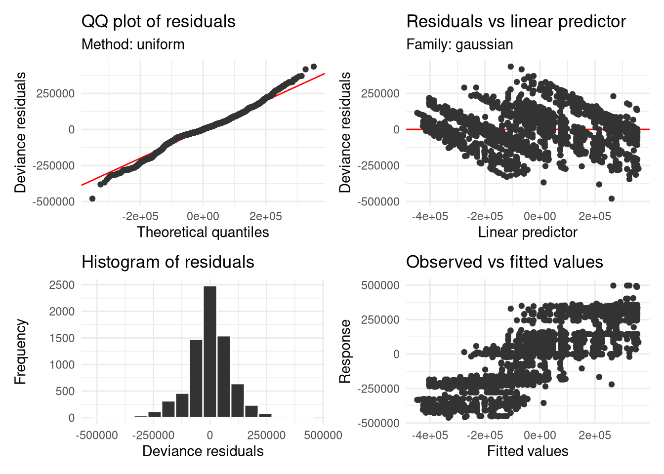
appraise(m2)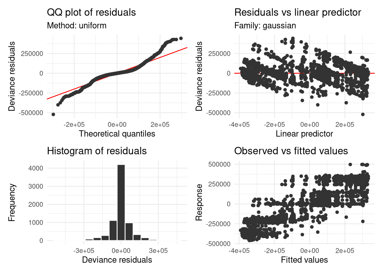
appraise(m1_mf)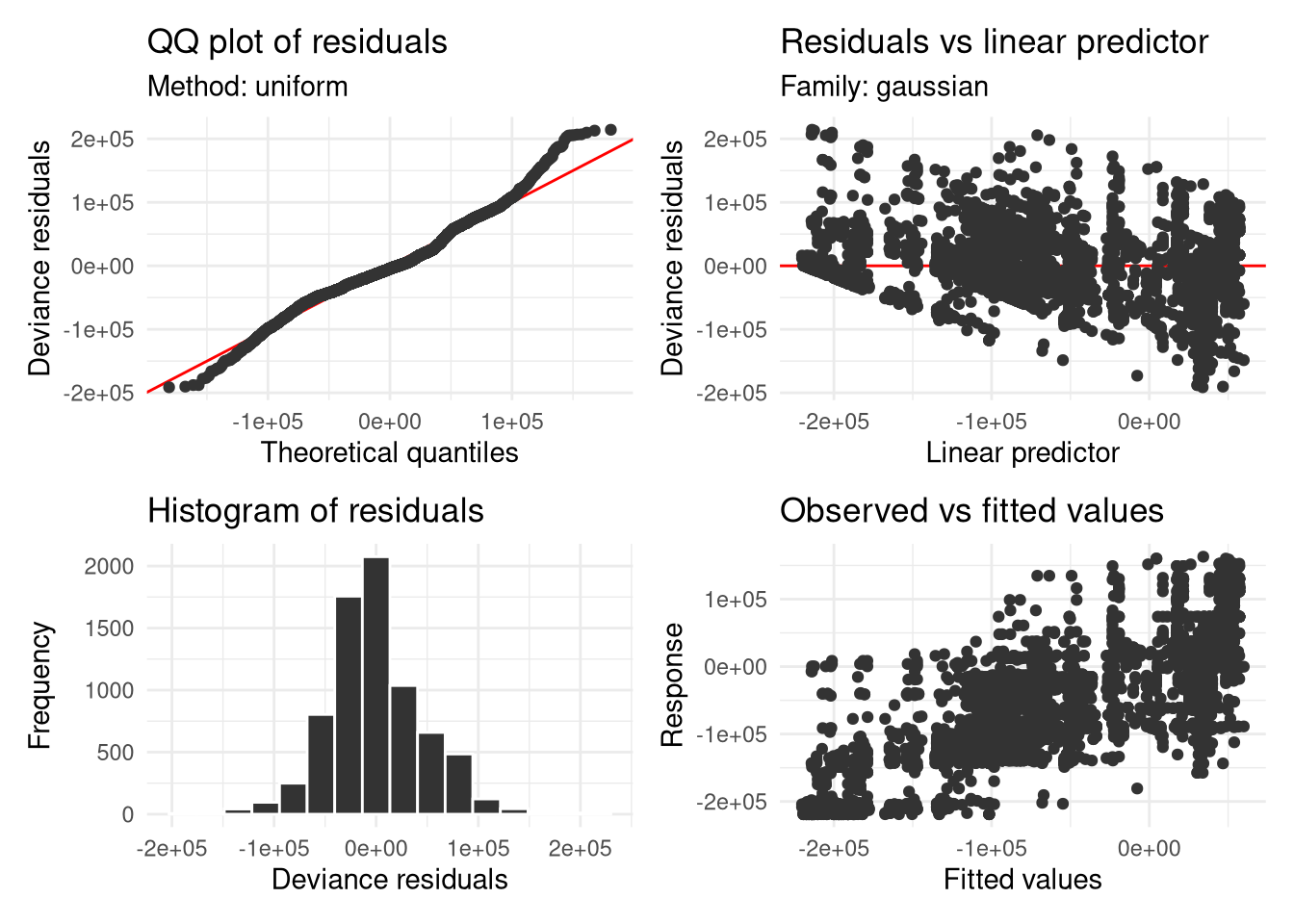
appraise(m2_mf)