4 Data cleaning

Author

Mike O’Brien

Published

May 1, 2026

library(arrow)
library(dplyr)
library(ggplot2)

5 Striped bass

sb <- open_dataset("../data/RAW/combined_striped_bass.parquet") |>
  filter(longitude != 0, !is.na(datetime)) |> # CHANGE THIS LATER!
  mutate(latitude = abs(latitude), wk = week(datetime)) |>
  group_by(transmitter, year, wk, group) |>
  summarize(
    med_lon = median(longitude, na.rm = TRUE),
    med_lat = median(latitude, na.rm = TRUE)
  ) |>
  collect()

First visualize the distribution of the median per-individual latitudes through time:

ggplot(sb) +
  geom_point(aes(x = wk, y = med_lat, color = group), alpha = 0.4) +
  facet_wrap(~year) +
  labs(x = "Week of year", y = "Weekly median latitude") +
  theme_minimal() +
  theme(axis.title = element_text(size = 12))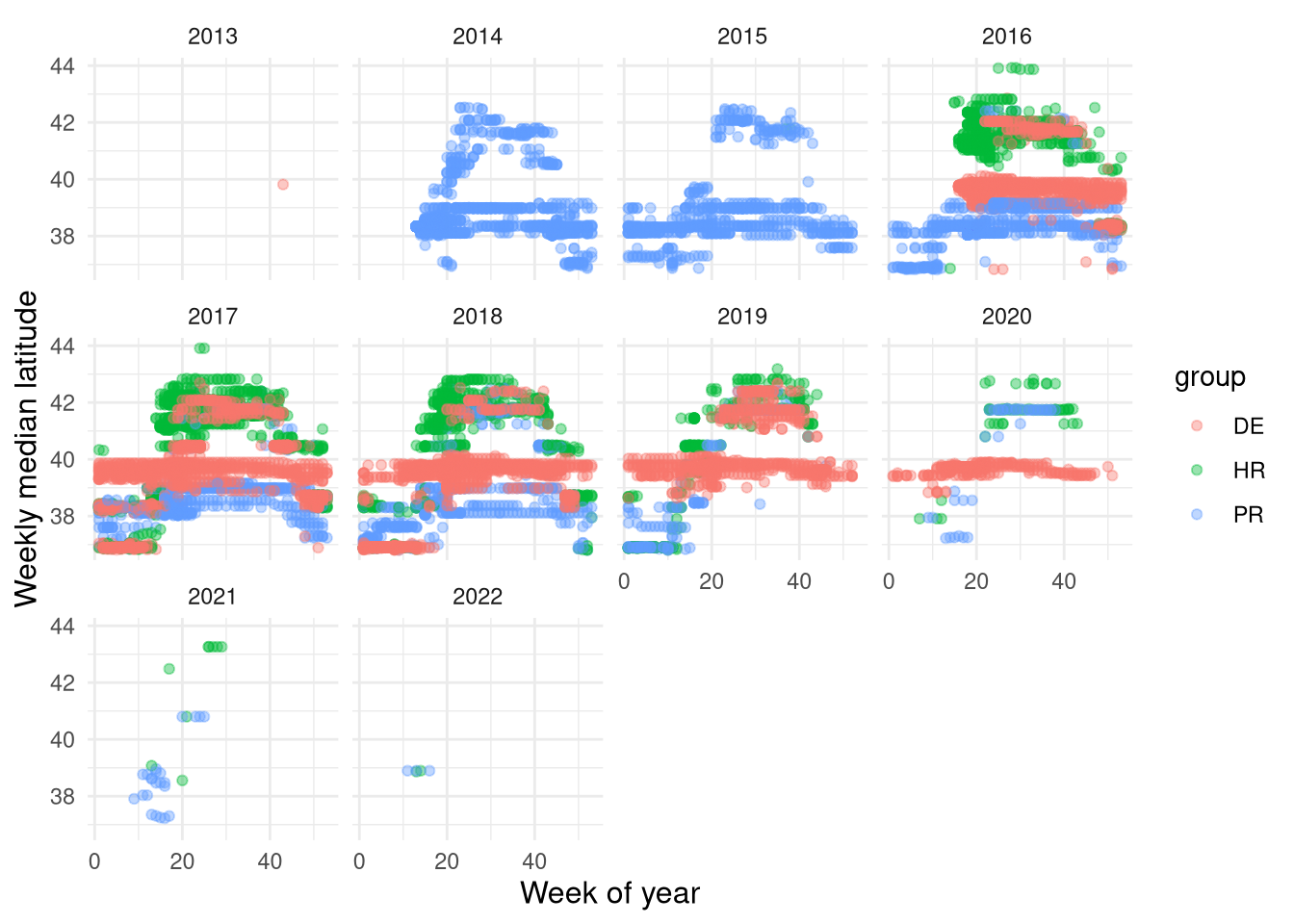

Weekly median latitude of striped bass. Colors represent putative populations; DE: Delaware, HR: Hudson River, PR: Potomac River.

It seems that we have resident striped bass from both the Delaware and Potomac River. Striped bass exhibit partial migration, where fish <80 cm remain resident in their natal estuary (Secor et al. 2020) (though our understanding of this is rapidly changing!). The projects providing the data for Delaware and Potomac fish purposefully tagged smaller, resident fish. As a first pass, we’ll remove any fish that didn’t move higher than 40.46 \(\degree\) latitude (the latitude of Trenton, NJ).

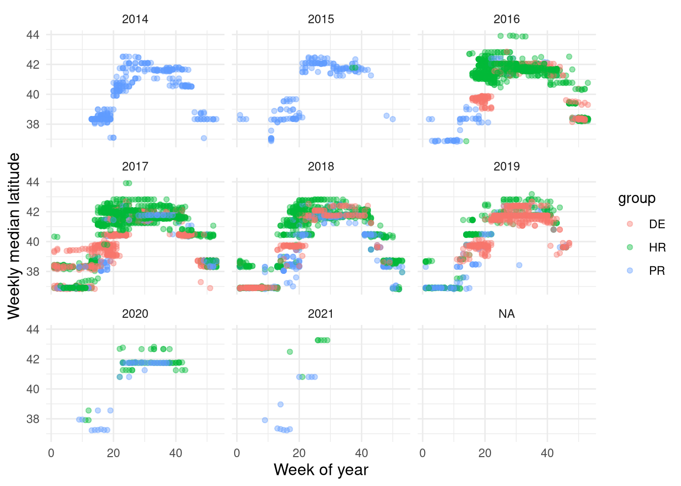
Great, now we definitely have some migratory striped bass.

open_dataset("data/RAW/combined_striped_bass.parquet") |>
  anti_join(drop) |>
  mutate(latitude = abs(latitude), wk = week(datetime)) |>
  write_parquet("data/derived/striped_bass.parquet")