8  Accessing Environmental Covariates

This chapter tracks the provenance of, and access to, environmental covariates. Depth, sea surface temperature, and chlorophyll a data are location specific and thus specific to the location dataset that is being used. We will use weekly median positions of striped bass as an example location dataset in those instances, but data for other species will be processed similarly.

library(arrow)
library(dplyr)
library(tidyr)
library(ggplot2)
library(sf)
library(terra)

set_theme(theme_minimal())

sb_file <- file.path(
  Sys.getenv("DATA_DIR"),
  "data/derived/striped_bass.parquet"
)

sb <- open_dataset(sb_file) |>
  filter(latitude > 34) |> # detections almost definitely wrong and needs to be removed
  group_by(transmitter, year, wk) |>
  summarize(
    med_lon = median(longitude, na.rm = TRUE),
    med_lat = median(latitude, na.rm = TRUE)
  ) |>
  ungroup() |>
  distinct(med_lon, med_lat, year, wk) |>
  collect()

9 Direct download

9.1 North Atlantic Oscillation (NAO)

The NAO index can be accessed at the National Weather Service’s Climate Prediction Center.

nao <- "https://ftp.cpc.ncep.noaa.gov/cwlinks/norm.daily.nao.cdas.z500.19500101_current.csv" |>
  read.csv()
write.csv(nao, "data/RAW/nao.csv", row.names = FALSE)

nao <- read.csv(
  file.path(
    Sys.getenv("DATA_DIR"),
    "data/RAW/nao.csv"
  )
)
summary(nao)

      year          month             day        nao_index_cdas    
 Min.   :1950   Min.   : 1.000   Min.   : 1.00   Min.   :-3.25400  
 1st Qu.:1969   1st Qu.: 4.000   1st Qu.: 8.00   1st Qu.:-0.53000  
 Median :1988   Median : 7.000   Median :16.00   Median : 0.05700  
 Mean   :1988   Mean   : 6.512   Mean   :15.73   Mean   : 0.02635  
 3rd Qu.:2007   3rd Qu.:10.000   3rd Qu.:23.00   3rd Qu.: 0.60774  
 Max.   :2026   Max.   :12.000   Max.   :31.00   Max.   : 2.75132  
                                                 NAs    :2         

ggplot(nao) +
  geom_line(
    aes(
      x = as.Date(sprintf("%d-%02d-%02d", year, month, day)),
      y = nao_index_cdas
    )
  ) +
  labs(x = NULL, y = "NAO Index")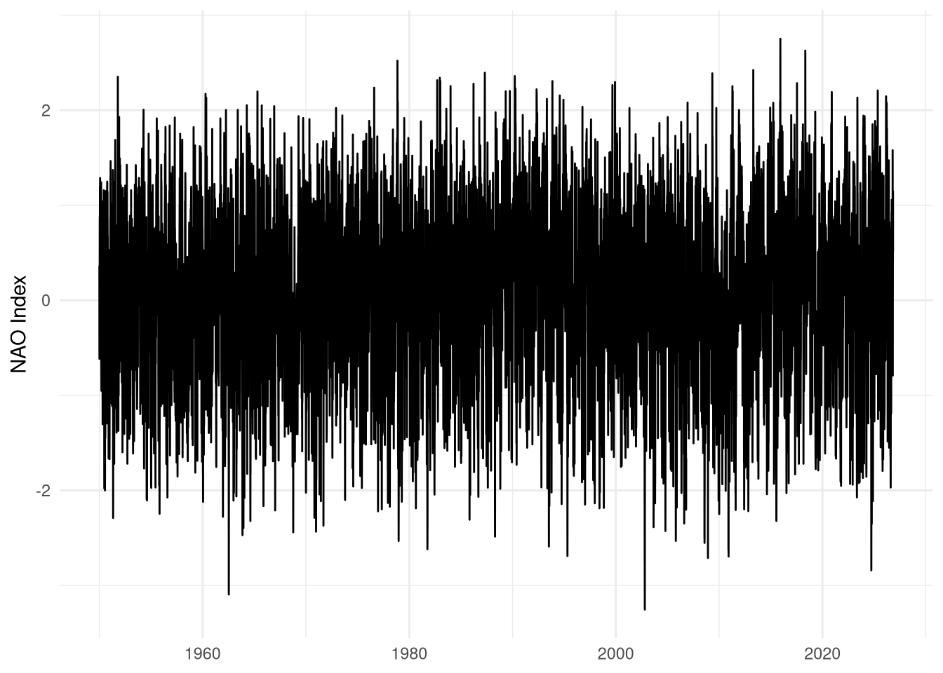

9.2 Gulf Stream Index

Gulf Stream Indices are available through the ecodata package (Beltz et al. 2026), “R data package developed by the Ecosystems Dynamics and Assessment Branch of the Northeast Fisheries Science Center for use in State of the Ecosystem (SOE) reporting”. The whole package can be installed, but we’ll just grab the source data directly.

download.file(
  "https://github.com/NOAA-EDAB/ecodata/raw/refs/heads/main/data/gsi.rda",
  "data/RAW/gsi.rda"
)

load(file.path(
  Sys.getenv("DATA_DIR"),
  "data/RAW/gsi.rda"
))

9.2.1 Gulf Stream Index

gsi |>
  filter(Var == "gulf stream index") |>
  ggplot() +
  geom_line(
    aes(
      x = as.Date(paste0(Time, ".01"), format = "%Y.%m.%d"),
      y = Value
    )
  ) +
  labs(x = NULL, y = "Gulf Stream Index")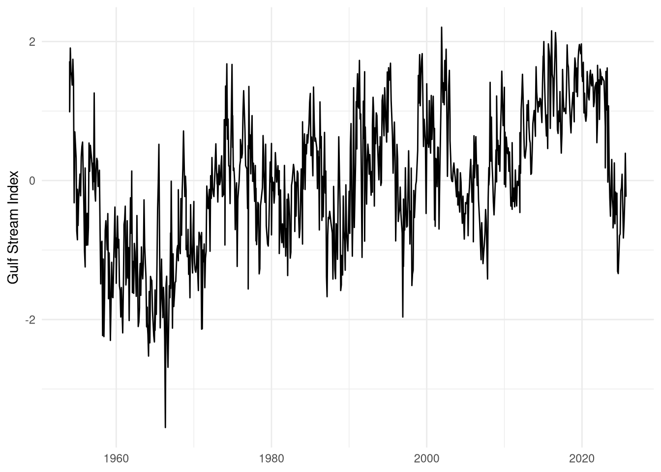

9.2.2 Western Gulf Stream Index

gsi |>
  filter(Var == "western gulf stream index") |>
  ggplot() +
  geom_line(
    aes(
      x = as.Date(paste0(Time, ".01"), format = "%Y.%m.%d"),
      y = Value
    )
  ) +
  labs(x = NULL, y = "Western Gulf Stream Index")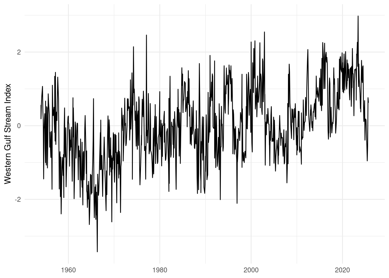

9.3 Depth

We accessed depth data from the coastal relief model provided by the NOAA National Centers for Environmental Information (Coastal Relief Models (CRMs), n.d.). Data are at roughly 30\(m^2\) resolutions and split across three volumes: one for the northeast US, one for the southeast US, and one for Florida and the Gulf of Mexico.

base_url <- "NETCDF:https://www.ngdc.noaa.gov/thredds/dodsC/crm/cudem/crm_vol%i_2023.nc"

9.3.1 Northeast Atlantic

depth_ne <- rast(sprintf(base_url, 1))
depth_ne

class       : SpatRaster
size        : 25200, 43200, 1  (nrow, ncol, nlyr)
dimensions  : lon, lat (43200, 25200}
resolution  : 0.0002777778, 0.0002777778  (x, y)
extent      : -77, -65, 39, 46  (xmin, xmax, ymin, ymax)
coord. ref. : lon/lat WGS 84 (EPSG:4326)
source      : crm_vol1_2023.nc
varname     : z (z)
name        : z
unit        : meters

plot(depth_ne, maxcell = 2000, col = terrain.colors(100))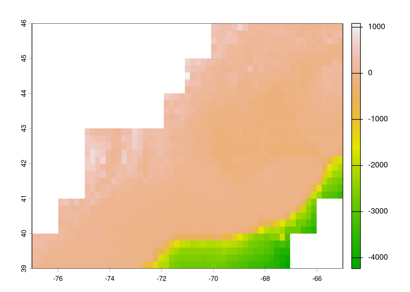

9.3.2 Southeast Atlantic

depth_se <- rast(sprintf(base_url, 2))
depth_se

class       : SpatRaster
size        : 25200, 54000, 1  (nrow, ncol, nlyr)
dimensions  : lon, lat (54000, 25200}
resolution  : 0.0002777778, 0.0002777778  (x, y)
extent      : -83, -68, 32, 39  (xmin, xmax, ymin, ymax)
coord. ref. : lon/lat WGS 84 (EPSG:4326)
source      : crm_vol2_2023.nc
varname     : z (z)
name        : z
unit        : meters

plot(depth_se, maxcell = 2000, col = terrain.colors(100))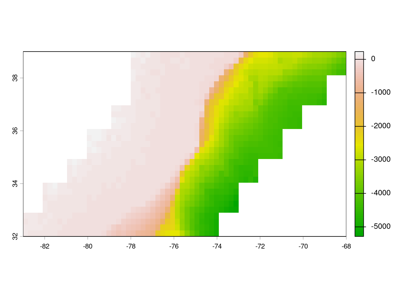

9.3.3 Florida and Gulf of Mexico

depth_fl <- rast(sprintf(base_url, 3))
depth_fl

class       : SpatRaster
size        : 28800, 28800, 1  (nrow, ncol, nlyr)
dimensions  : lon, lat (28800, 28800}
resolution  : 0.0002777778, 0.0002777778  (x, y)
extent      : -84, -76, 24, 32  (xmin, xmax, ymin, ymax)
coord. ref. : lon/lat WGS 84 (EPSG:4326)
source      : crm_vol3_2023.nc
varname     : z (z)
name        : z
unit        : meters

plot(depth_fl, maxcell = 2000, col = terrain.colors(100))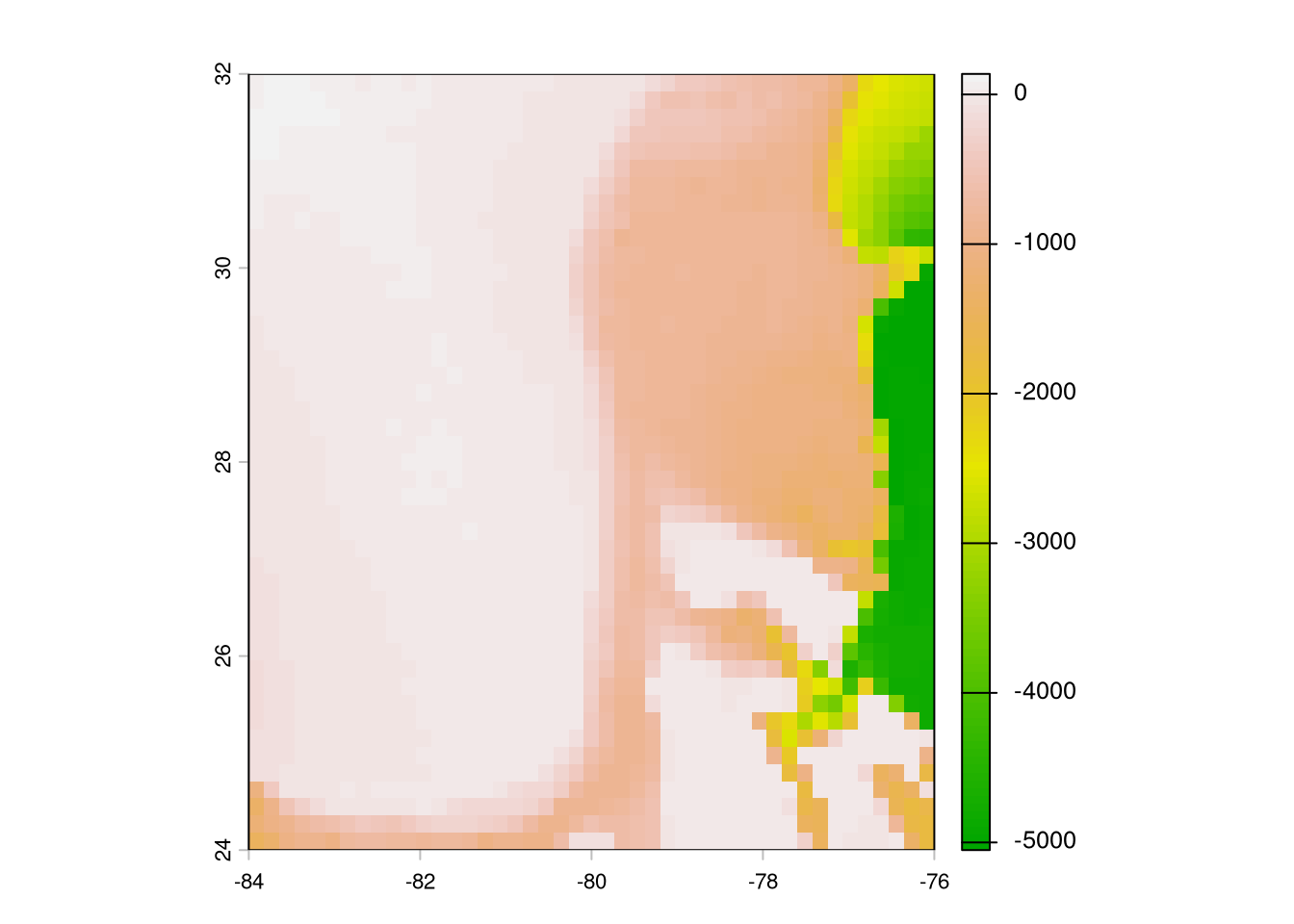

9.4 Sea surface temperature

9.4.1 Ocean temperature

(GHRSST Level 4 MUR Global Foundation Sea Surface Temperature Analysis (V4.1) 2015)

Query needs date, latitude, and longitude. Right now we are using median position per week. Rather than just picking one day in the given week, we’ll take the mean SST at each position for the week.

sb_wk <- sb |>
  filter(!is.na(year)) |>
  mutate(
    start_date = as.Date(paste(year, 1, 1, sep = "-")) + (wk - 1) * 7
  ) |>
  uncount(7, .id = 'day') |>
  mutate(date = start_date + day - 1, date = as.POSIXct(date)) |>
  filter(year == 2014) |> #!!!
  select(med_lon, med_lat, date) |>
  arrange(date)

Code

extract_ghrsst.py

#!/usr/bin/env python3
# /// script
# dependencies = [
#   "pandas",
#   "xarray",
#   "zarr",
#   "dask",
#   "s3fs",
#   "fsspec",
# ]
# ///

import sys
import argparse
import pandas as pd
import xarray as xr
import dask

def main():
    parser = argparse.ArgumentParser(description="Extract JPL MUR SST v4.1 data for spatial points.")
    parser.add_argument("-i", "--input", default=sys.stdin, help="Input CSV file path (default: stdin)")
    parser.add_argument("-o", "--output", default=sys.stdout, help="Output CSV file path (default: stdout)")
    parser.add_argument("-w", "--workers", type=int, default=16, help="Number of Dask thread workers (default: 16)")
    args = parser.parse_args()

    # 1. Read input dataset
    df = pd.read_csv(args.input)
    df['date'] = pd.to_datetime(df["date"])

    # 2. Open S3 Zarr store
    sys.stderr.write("Opening S3 Zarr store...\n")
    ds = xr.open_zarr(
      "s3://mur-sst/zarr-v1",
      storage_options = {
        "anon": True,
        "client_kwargs": {"region_name": "us-west-2"},
        "default_fill_cache": False
      }, 
      consolidated = True
    )

    # Spatial bounding box (+/- 0.02 deg buffer)
    min_lat, max_lat = df['med_lat'].min() - 0.02, df['med_lat'].max() + 0.02
    min_lon, max_lon = df['med_lon'].min() - 0.02, df['med_lon'].max() + 0.02

    results = []

    for yr, sub_df in df.groupby(df['date'].dt.year):
        sub_df = sub_df.copy()
        unique_dates = sub_df['date'].drop_duplicates().sort_values().values
        
        sys.stderr.write(f"Processing {yr}: {len(unique_dates)} dates, {len(sub_df)} rows...\n")

        with dask.config.set(scheduler='threads', num_workers=args.workers):
            cube = (
                ds['analysed_sst']
                .sel(lat=slice(min_lat, max_lat), lon=slice(min_lon, max_lon))
                .sel(time=unique_dates, method="nearest")
                .load()
            )

        extracted = cube.sel(
            time = xr.DataArray(sub_df['date'].values, dims="points"),
            lat = xr.DataArray(sub_df['med_lat'].values, dims="points"),
            lon = xr.DataArray(sub_df['med_lon'].values, dims="points"),
            method = 'nearest'
        )

        sub_df['sst_celsius'] = (extracted - 273.15).values
        results.append(sub_df)

    final_df = pd.concat(results, ignore_index=True)

    final_df['year'] = final_df['date'].dt.year
    final_df['wk'] = ((final_df['date'].dt.day_of_year - 1) // 7) + 1
    final_df = final_df.groupby(['med_lat', 'med_lon', 'year', 'wk']).agg(
        sst_celsius=('sst_celsius', 'mean')
    ).reset_index()


    final_df.to_csv(args.output, index=False)

if __name__ == "__main__":
    main()

sb_sst <- read.csv(
  file.path(
    Sys.getenv("DATA_DIR"),
    "data/derived/sb_sst.csv"
  )
)
head(sb_sst)

   med_lat   med_lon year wk sst_celsius
1 37.06356 -76.09292 2014 49   10.173571
2 37.09695 -75.99200 2014 19   17.681143
3 37.09695 -75.99200 2014 20   18.886571
4 38.03300 -76.33550 2014 16   10.601143
5 38.03327 -76.33706 2014 14    7.361429
6 38.03327 -76.33706 2014 16   10.601143

9.4.2 Estuary temperature

Atlantic sturgeon and striped bass are anadromous species and so spend 1-2 months per year in estuaries. Unfortunately, observing system products do not usually resolve to the small spatial scales characteristic of spawning estuaries. We plan to use NOAA CO-OPs station data from within each estuary, with the assumption that these temperatures will represent the entire system.

9.5 Chlorophyll a

10 Derived data

10.1 Distance from shore

We derived distance from shore by calculating the Euclidean distance between weekly median locations in the rotated plane and the similarly-rotated Natural Earth 1:110m land polygon. We used the sf::st_distance for these calculations.

download.file(
  "https://naciscdn.org/naturalearth/110m/physical/ne_110m_land.zip",
  "data/RAW/ne_110.zip"
)

land <- st_read(file.path(
  "/vsizip",
  Sys.getenv("DATA_DIR"),
  "data/RAW/ne_110.zip"
))

Reading layer `ne_110m_land' from data source `/vsizip/../../data/RAW/ne_110.zip' using driver `ESRI Shapefile'
Simple feature collection with 127 features and 3 fields
Geometry type: POLYGON
Dimension:     XY
Bounding box:  xmin: -180 ymin: -90 xmax: 180 ymax: 83.64513
Geodetic CRS:  WGS 84

ggplot(land) +
  geom_sf()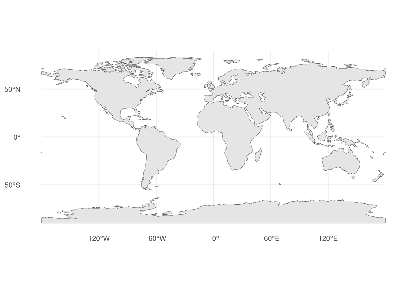

rotated_projection <- open_dataset(sb_file) |>
  filter(longitude != 0) |> # Idiosyncrasy of this data, will be changed.
  mutate(latitude = abs(latitude)) |> # Idiosyncrasy of this data, will be changed.
  distinct(latitude, longitude) |>
  summarize(
    lon0 = median(longitude, na.rm = TRUE),
    lat0 = median(latitude, na.rm = TRUE)
  ) |>
  collect() |>
  (\(.) {
    paste0(
      "+proj=aeqd +lon_0=",
      round(.$lon0, 3),
      " +lat_0=",
      round(.$lat0, 3)
    )
  })()

sb_positions <- open_dataset(sb_file) |>
  filter(latitude > 34) |> # detections almost definitely wrong and needs to be removed
  group_by(transmitter, year, wk, group) |>
  summarize(
    med_lon = median(longitude, na.rm = TRUE),
    med_lat = median(latitude, na.rm = TRUE)
  ) |>
  ungroup() |>
  distinct(med_lon, med_lat) |>
  collect() |>
  st_as_sf(coords = c("med_lon", "med_lat"), crs = 4326) |>
  st_transform(rotated_projection)

land <- land |>
  st_transform(rotated_projection)

ggplot(land) +
  geom_sf()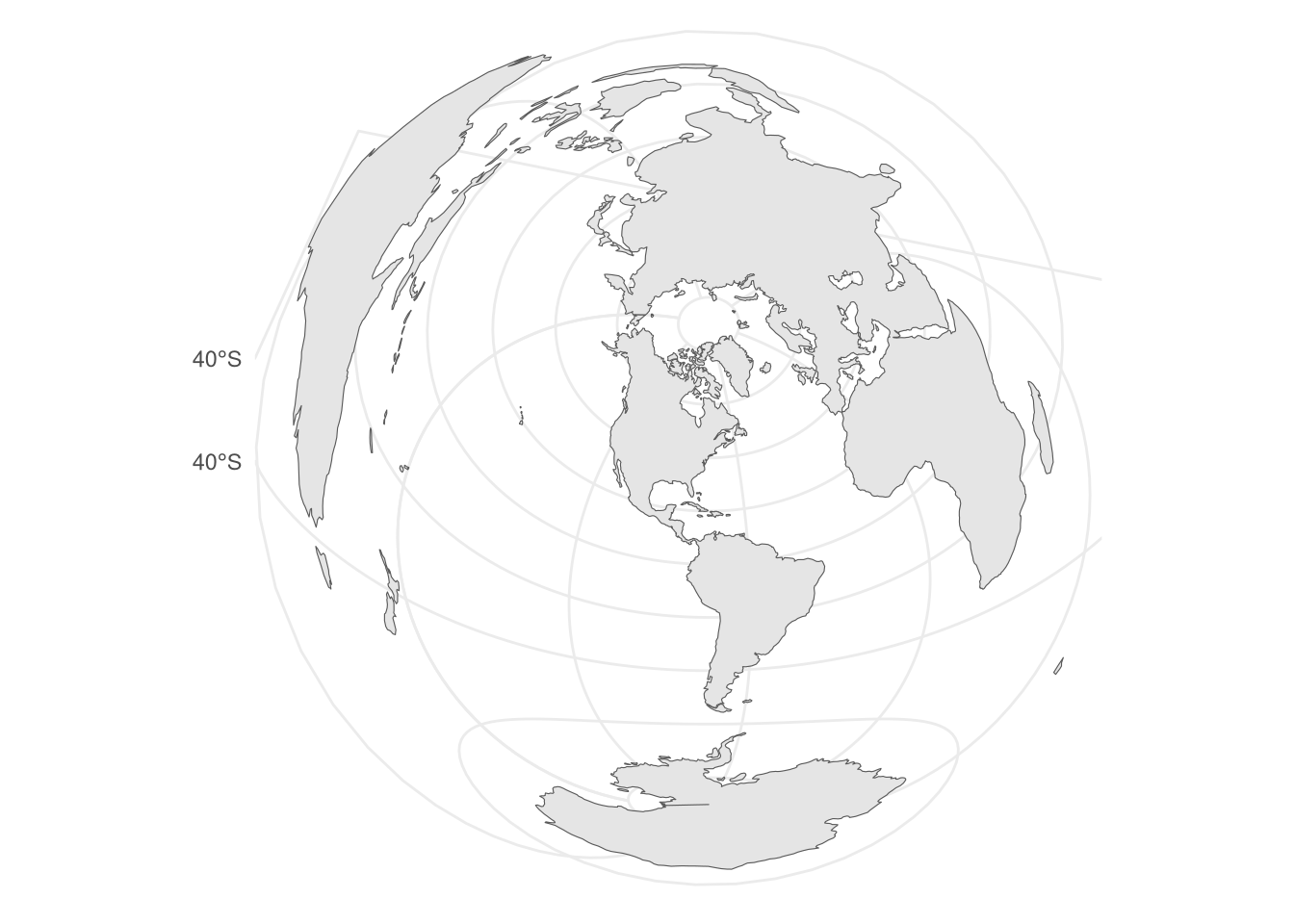

dists <- st_distance(sb_positions, st_combine(land))

ggplot(data.frame(dist = as.numeric(dists))) +
  geom_histogram(aes(x = dist))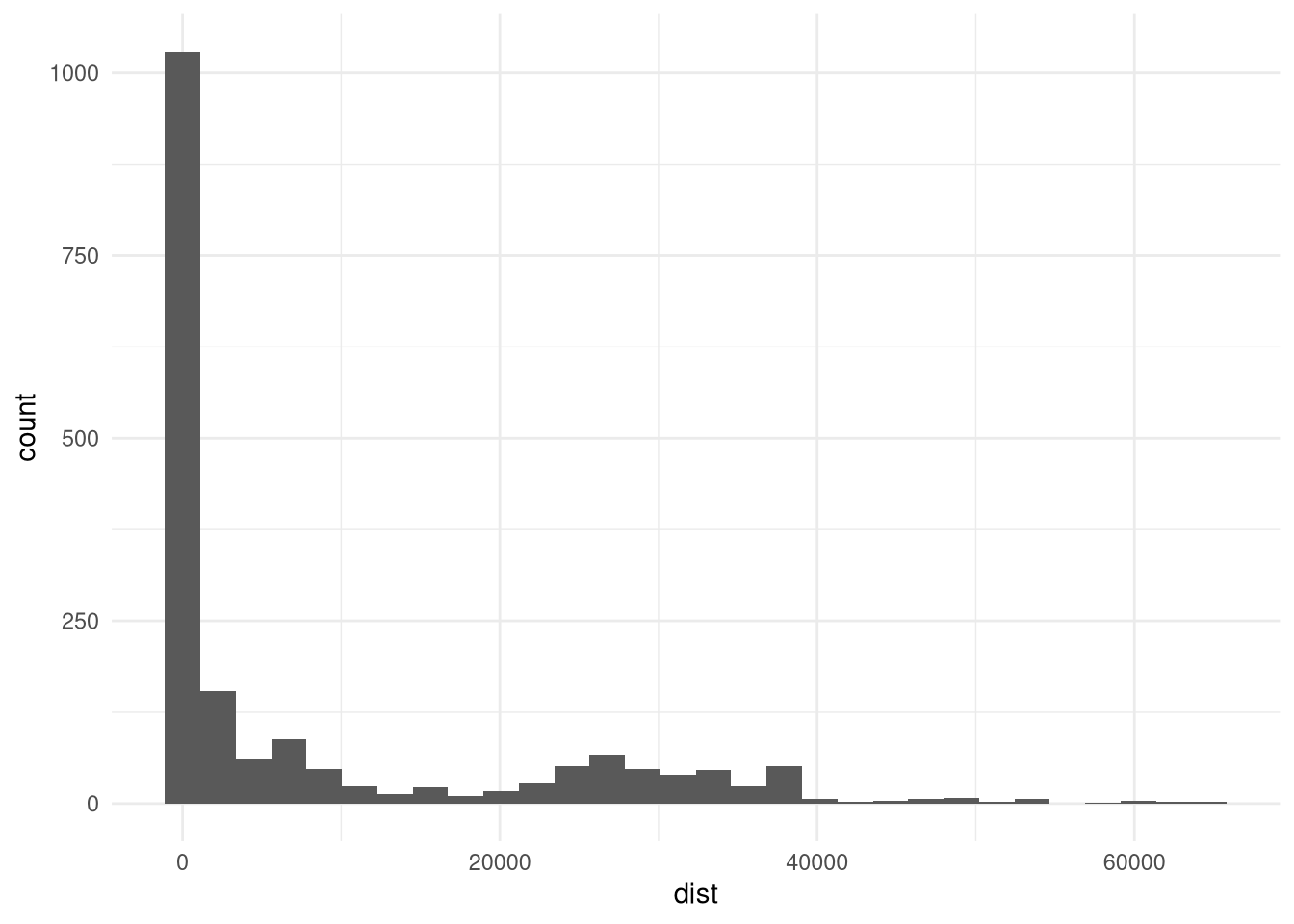

10.2 Change in chloropyll a

We derived change in chlorophyll a from the data downloaded in Section 9.5.

10.3 Change in sea surfance temperature

We derived change in sea surface temperature from the data downloaded in Section 9.4.

Beltz, Brandon, Andy Beet, Kimberly Bastille, and Sean Hardison. 2026. Ecodata: Documentation of Ecosystem Indicator Reporting. https://noaa-edab.github.io/ecodata/.

Coastal Relief Models (CRMs). n.d. https://doi.org/10.25921/5ZN5-KN44.

GHRSST Level 4 MUR Global Foundation Sea Surface Temperature Analysis (V4.1). 2015. NASA. http://podaac.jpl.nasa.gov/dataset/MUR-JPL-L4-GLOB-v4.1.